1 Intro

We have some Tongan smart meter data provided as part of Kakau Foliaki’s PhD. This code loads & tests it.

2 Initial dataset - file: CRF_2020_1_28_4296268_1 - Copy.7z

Sent to KF. No meta-data. Sent as xml. Converted (possibly with errors) to .csv.

In theory this should be half-hourly electricity consumption (Wh or kWh) data for a large(ish) number of Tongan households. It even be all Tongan households with smart meters. But who knows…

What have we got?

f1_xml <- path.expand(paste0(dPath, "/CRF_2020_1_28_4296268_1 - Copy.xml"))
f1_csv <- path.expand(paste0(dPath, "/Smartmeter.csv.gz"))

First try loading the (huge) xml file (/Volumes/hum-csafe/Research Projects/FoliakiPhD/smartMeterData/v1/CRF_2020_1_28_4296268_1 - Copy.xml)

Skip this - take ages & fails

#try(f1_df <- XML::xmlToDataFrame(f1_xml)) # try as it breaks if there's an error

Helpful.

Now try loading the .csv file (/Volumes/hum-csafe/Research Projects/FoliakiPhD/smartMeterData/v1/Smartmeter.csv.gz) and test what we get before any processing.

f1_dt_orig <- data.table::fread(f1_csv, check.names = TRUE)

# names of variables
names(f1_dt_orig)

##  [1] "EndDate"                                                                                                                        
##  [2] "IntervalLength"                                                                                                                 
##  [3] "StartDate"                                                                                                                      
##  [4] "X.id"                                                                                                                           
##  [5] "EndPointChannelID"                                                                                                              
##  [6] "NumberOfReadings"                                                                                                               
##  [7] "X.id.1"                                                                                                                         
##  [8] "EndTime"                                                                                                                        
##  [9] "NumberOfReadings.1"                                                                                                             
## [10] "Value"                                                                                                                          
## [11] "X.id.2"                                                                                                                         
## [12] "X.Channels.Channel.ContiguousIntervalSets.ContiguousIntervalSet.Readings.Reading.ReadingStatus.UnencodedStatus.StatusCodes.Code"
## [13] "X.Channels.Channel.OptionalChannelDatas.OptionalChannelData..Value"                                                             
## [14] "X.Channels.Channel.OptionalChannelDatas.OptionalChannelData..Value..agg"                                                        
## [15] "X.Header.CorrelationID..Id"                                                                                                     
## [16] "X.Header.CorrelationID..Id..agg"

h <- head(f1_dt_orig)
kableExtra::kable(h, caption = "First few rows")

(#tab:load_f1_csv)First few rows
EndDate	IntervalLength	StartDate	X.id	EndPointChannelID	NumberOfReadings	X.id.1	EndTime	NumberOfReadings.1	Value	X.id.2	X.Channels.Channel.OptionalChannelDatas.OptionalChannelData..Value	X.Channels.Channel.OptionalChannelDatas.OptionalChannelData..Value..agg	X.Header.CorrelationID..Id	X.Header.CorrelationID..Id..agg
27/01/20 21:25	30	30/11/18 11:00	1	318314893:1	816	1	12/05/2019 05:00:00	11/18/2019 05:00:00	235	1	14	14	4296268	4296268
27/01/20 21:25	30	30/11/18 11:00	1	318314893:1	816	1	12/05/2019 05:00:00	11/18/2019 05:00:00	235	2	14	NA	4296268	NA
27/01/20 21:25	30	30/11/18 11:00	1	318314893:1	816	1	12/05/2019 05:00:00	11/18/2019 05:00:00	233	3	14	NA	4296268	NA
27/01/20 21:25	30	30/11/18 11:00	1	318314893:1	816	1	12/05/2019 05:00:00	11/18/2019 05:00:00	231	4	14	NA	4296268	NA
27/01/20 21:25	30	30/11/18 11:00	1	318314893:1	816	1	12/05/2019 05:00:00	11/18/2019 05:00:00	234	5	14	NA	4296268	NA
27/01/20 21:25	30	30/11/18 11:00	1	318314893:1	816	1	12/05/2019 05:00:00	11/18/2019 05:00:00	234	6	14	NA	4296268	NA

sk <- skimr::skim(f1_dt_orig)

print(sk)

## ── Data Summary ────────────────────────
##                            Values    
## Name                       f1_dt_orig
## Number of rows             1048574   
## Number of columns          16        
## _______________________              
## Column type frequency:               
##   character                6         
##   numeric                  10        
## ________________________             
## Group variables            None      
## 
## ── Variable type: character ────────────────────────────────────────────────────
##   skim_variable                                                                 
## 1 EndDate                                                                       
## 2 StartDate                                                                     
## 3 EndPointChannelID                                                             
## 4 EndTime                                                                       
## 5 NumberOfReadings.1                                                            
## 6 X.Channels.Channel.ContiguousIntervalSets.ContiguousIntervalSet.Readings.Read…
##   n_missing complete_rate   min   max   empty n_unique whitespace
## 1         0             1     0    14   11155        2          0
## 2         0             1     0    14   11155        2          0
## 3         0             1    11    11       0      300          0
## 4         0             1     0    19 1047722        2          0
## 5         0             1     0    19 1047722        2          0
## 6         0             1     0    19  976345        7          0
## 
## ── Variable type: numeric ──────────────────────────────────────────────────────
##    skim_variable                                                          
##  1 IntervalLength                                                         
##  2 X.id                                                                   
##  3 NumberOfReadings                                                       
##  4 X.id.1                                                                 
##  5 Value                                                                  
##  6 X.id.2                                                                 
##  7 X.Channels.Channel.OptionalChannelDatas.OptionalChannelData..Value     
##  8 X.Channels.Channel.OptionalChannelDatas.OptionalChannelData..Value..agg
##  9 X.Header.CorrelationID..Id                                             
## 10 X.Header.CorrelationID..Id..agg                                        
##    n_missing complete_rate     mean       sd      p0      p25     p50      p75
##  1     11155   0.989            30       0        30      30       30      30 
##  2         0   1               300.    173.        1     149      299     449 
##  3     11155   0.989          1524.    679.       12     816     1896    1896 
##  4     11155   0.989           447.    259.        1     221      460     672 
##  5     11155   0.989           232.     32.1       0     234      237     240 
##  6     11155   0.989        503715. 290824.        1  251860.  503705  755582.
##  7         0   1                14       0        14      14       14      14 
##  8   1047975   0.000571         14       0        14      14       14      14 
##  9         0   1           4296268       0   4296268 4296268  4296268 4296268 
## 10   1048573   0.000000954 4296268      NA   4296268 4296268  4296268 4296268 
##       p100 hist 
##  1      30 ▁▁▇▁▁
##  2     599 ▇▇▇▇▇
##  3    2724 ▁▇▁▇▂
##  4     895 ▇▆▇▆▇
##  5     917 ▁▇▁▁▁
##  6 1007419 ▇▇▇▇▇
##  7      14 ▁▁▇▁▁
##  8      14 ▁▁▇▁▁
##  9 4296268 ▁▁▇▁▁
## 10 4296268 ▁▁▇▁▁

So what does all that mean? Let’s test some of the variables.

f1_dt <- data.table::copy(f1_dt_orig) # so we can revert if needed

2.1 StartDate

Looks like a dateTime, does it walk like a dateTime? Looks like it’s in d/m/y H:M form.

f1_dt[, ba_StartDate := lubridate::dmy_hm(StartDate)]

# convert & test

head(f1_dt[, .(StartDate, ba_StartDate)])

##         StartDate        ba_StartDate
## 1: 30/11/18 11:00 2018-11-30 11:00:00
## 2: 30/11/18 11:00 2018-11-30 11:00:00
## 3: 30/11/18 11:00 2018-11-30 11:00:00
## 4: 30/11/18 11:00 2018-11-30 11:00:00
## 5: 30/11/18 11:00 2018-11-30 11:00:00
## 6: 30/11/18 11:00 2018-11-30 11:00:00

skimr::skim(f1_dt[, .(StartDate, ba_StartDate)])

(#tab:process_f1_csv_StartDate)Data summary

Name	f1_dt[, .(StartDate, ba_S…
Number of rows	1048574
Number of columns	2
_______________________
Column type frequency:
character	1
POSIXct	1
________________________
Group variables	None

Variable type: character

skim_variable	n_missing	complete_rate	min	max	empty	n_unique	whitespace
StartDate	0	1	0	14	11155	2	0

Variable type: POSIXct

skim_variable	n_missing	complete_rate	min	max	median	n_unique
ba_StartDate	11155	0.99	2018-11-30 11:00:00	2018-11-30 11:00:00	2018-11-30 11:00:00	1

So startDate is 2018-11-30 11:00:00 and is constant. Presumably this is the start date for the data extract?

2.2 EndDate

Logic (haha) would suggest this would be the end date for the data extract. Looks like it’s in d/m/y H:M form.

f1_dt[, ba_EndDate := lubridate::dmy_hm(EndDate)]
dt <- f1_dt[, .(EndDate, ba_EndDate)]
head(dt)

##           EndDate          ba_EndDate
## 1: 27/01/20 21:25 2020-01-27 21:25:00
## 2: 27/01/20 21:25 2020-01-27 21:25:00
## 3: 27/01/20 21:25 2020-01-27 21:25:00
## 4: 27/01/20 21:25 2020-01-27 21:25:00
## 5: 27/01/20 21:25 2020-01-27 21:25:00
## 6: 27/01/20 21:25 2020-01-27 21:25:00

skimr::skim(dt)

(#tab:process_f1_csv_EndDate)Data summary

Name	dt
Number of rows	1048574
Number of columns	2
_______________________
Column type frequency:
character	1
POSIXct	1
________________________
Group variables	None

Variable type: character

skim_variable	n_missing	complete_rate	min	max	empty	n_unique	whitespace
EndDate	0	1	0	14	11155	2	0

Variable type: POSIXct

skim_variable	n_missing	complete_rate	min	max	median	n_unique
ba_EndDate	11155	0.99	2020-01-27 21:25:00	2020-01-27 21:25:00	2020-01-27 21:25:00	1

And EndDate is also constant and is 2020-01-27 21:25:00 - but is not a round ‘half hour’?

2.3 EndTime

So what then is this? For a start it’s in a different form - d/m/y H:M:S

Of course it could also be m/d/y - can’t tell from these rows.

f1_dt[, ba_EndTime := lubridate::dmy_hms(EndTime)]
dt <- f1_dt[, .(EndTime, ba_EndTime)]
head(dt)

##                EndTime          ba_EndTime
## 1: 12/05/2019 05:00:00 2019-05-12 05:00:00
## 2: 12/05/2019 05:00:00 2019-05-12 05:00:00
## 3: 12/05/2019 05:00:00 2019-05-12 05:00:00
## 4: 12/05/2019 05:00:00 2019-05-12 05:00:00
## 5: 12/05/2019 05:00:00 2019-05-12 05:00:00
## 6: 12/05/2019 05:00:00 2019-05-12 05:00:00

skimr::skim(dt)

(#tab:process_f1_csv_EndTime)Data summary

Name	dt
Number of rows	1048574
Number of columns	2
_______________________
Column type frequency:
character	1
POSIXct	1
________________________
Group variables	None

Variable type: character

skim_variable	n_missing	complete_rate	min	max	empty	n_unique	whitespace
EndTime	0	1	0	19	1047722	2	0

Variable type: POSIXct

skim_variable	n_missing	complete_rate	min	max	median	n_unique
ba_EndTime	1047722	0	2019-05-12 05:00:00	2019-05-12 05:00:00	2019-05-12 05:00:00	1

So EndTime is also constant at 2019-05-12 05:00:00 but it is missing for a lot of rows.

2.4 NumberOfReadings_1

For some reason this looks like a dateTime too - are the column headings mis-aligned?

This is definitely in m/d/y H:M:S form…

f1_dt[, ba_NumberOfReadings.1 := lubridate::mdy_hms(NumberOfReadings.1)] #mdy?
dt <- f1_dt[, .(NumberOfReadings.1, ba_NumberOfReadings.1)]
head(dt)

##     NumberOfReadings.1 ba_NumberOfReadings.1
## 1: 11/18/2019 05:00:00   2019-11-18 05:00:00
## 2: 11/18/2019 05:00:00   2019-11-18 05:00:00
## 3: 11/18/2019 05:00:00   2019-11-18 05:00:00
## 4: 11/18/2019 05:00:00   2019-11-18 05:00:00
## 5: 11/18/2019 05:00:00   2019-11-18 05:00:00
## 6: 11/18/2019 05:00:00   2019-11-18 05:00:00

skimr::skim(dt)

(#tab:process_f1_csv_NumberOfReadings_1)Data summary

Name	dt
Number of rows	1048574
Number of columns	2
_______________________
Column type frequency:
character	1
POSIXct	1
________________________
Group variables	None

Variable type: character

skim_variable	n_missing	complete_rate	min	max	empty	n_unique	whitespace
NumberOfReadings.1	0	1	0	19	1047722	2	0

Variable type: POSIXct

skim_variable	n_missing	complete_rate	min	max	median	n_unique
ba_NumberOfReadings.1	1047722	0	2019-11-18 05:00:00	2019-11-18 05:00:00	2019-11-18 05:00:00	1

NumberOfReadings.1 is constant at 2019-11-18 05:00:00 with a lot of missing. So what is this?

We don’t seem to have an obvious half hourly dateTime field…

2.5 X.id* variables

Let’s look at the IDs.

h <- head(f1_dt[, .(X.id, X.id.1, X.id.2)], 10)
kableExtra::kable(h, caption = "IDs - example rows") %>%
  kable_styling()

Table 2.1: IDs - example rows
X.id	X.id.1	X.id.2
1	1	1
1	1	2
1	1	3
1	1	4
1	1	5
1	1	6
1	1	7
1	1	7
1	1	8
1	1	9

skimr::skim(f1_dt[, .(X.id, X.id.1, X.id.2)])

Table 2.1: Data summary

Name	f1_dt[, .(X.id, X.id.1, X…
Number of rows	1048574
Number of columns	3
_______________________
Column type frequency:
numeric	3
________________________
Group variables	None

Variable type: numeric

skim_variable	n_missing	complete_rate	mean	sd	p0	p25	p50	p75	p100	hist
X.id	0	1.00	299.83	173.13	1	149.0	299	449.0	599	▇▇▇▇▇
X.id.1	11155	0.99	446.71	259.02	1	221.0	460	672.0	895	▇▆▇▆▇
X.id.2	11155	0.99	503715.04	290824.01	1	251860.5	503705	755582.5	1007419	▇▇▇▇▇

So X.id and X.id1 could be true id variables. But X.id.2 seems to increase monotonically.

Unique values:

X.id: 599
X.id.1: 896
X.id.2: 1007420

2.5.1 X.id

# distributions
ggplot2::ggplot(f1_dt, aes(x = X.id)) +
  geom_histogram()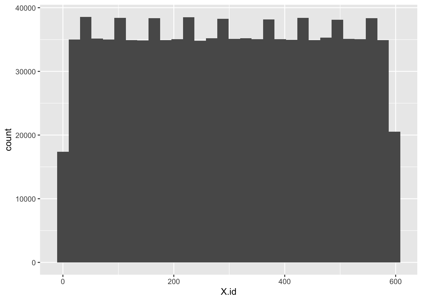

So what do we infer from that???

2.5.2 X.id.1

# distributions
ggplot2::ggplot(f1_dt, aes(x = X.id.1)) +
  geom_histogram()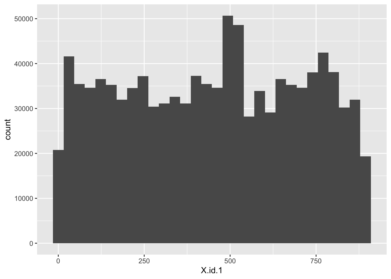

Well that looks more like a proper id - essentially random numbers of observations

2.5.3 X.id.2

# distributions
ggplot2::ggplot(f1_dt, aes(x = X.id.2)) +
  geom_histogram()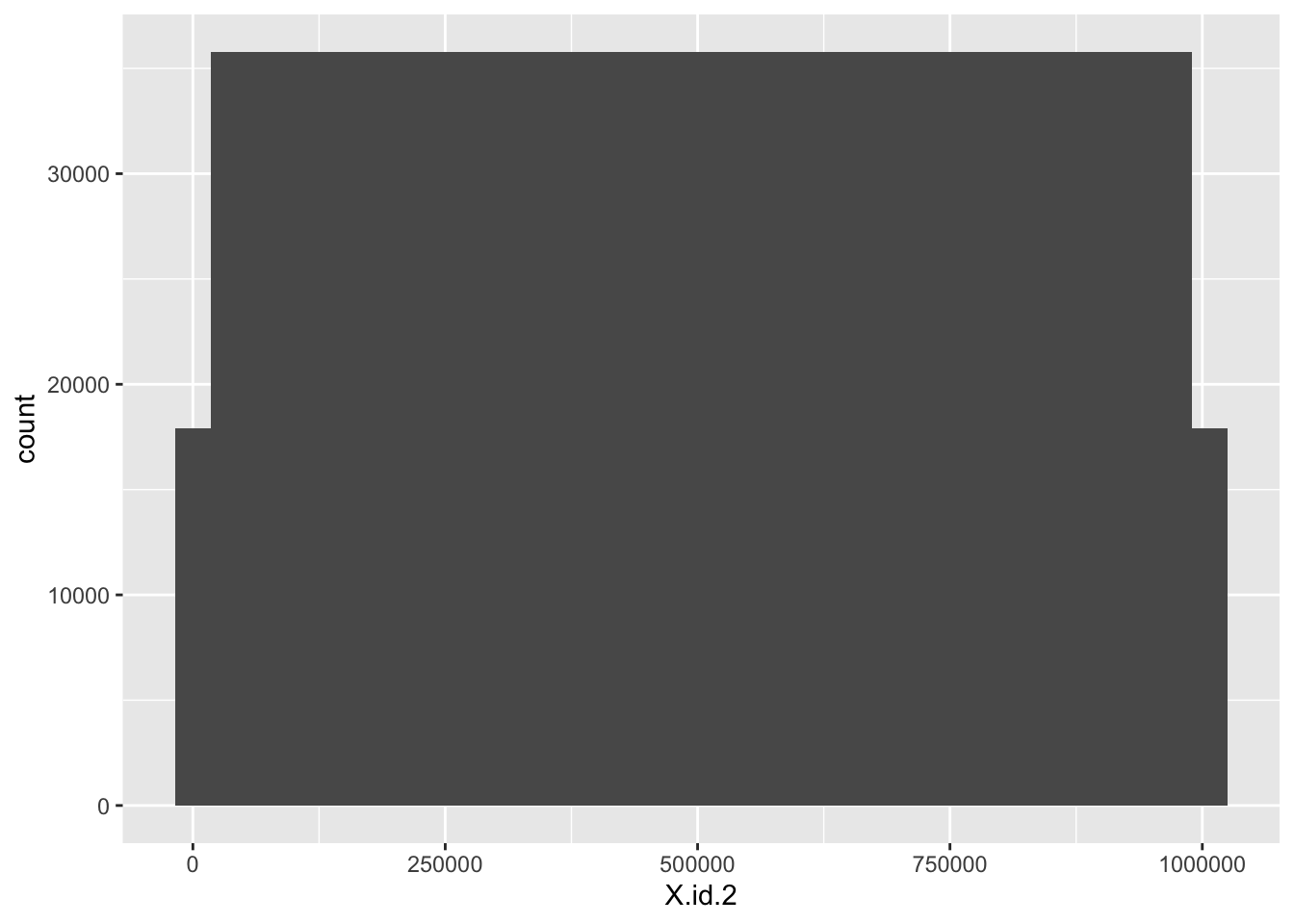

2.5.4 What the ID?

A summary table:

dt <- f1_dt[, .(nObs = .N,
                min_X.id = min(X.id),
                max_X.id = max(X.id),
                min_X.id.2 = min(X.id.2),
                max_X.id.2 = max(X.id.2)
                ), keyby = .(X.id.1)]

kableExtra::kable(head(dt), caption = "First few rows of summary table by X.id.1") %>%
  kable_styling()

(#tab:f1_id_summary)First few rows of summary table by X.id.1
X.id.1	nObs	min_X.id	max_X.id	min_X.id.2	max_X.id.2
NA	11155	2	598	NA	NA
1	852	1	1	1	816
2	1947	1	1	817	2712
3	661	1	1	2713	3360
4	853	3	3	3361	4176
5	1944	3	3	4177	6072

So:

X.id has 599 unique values but they have weird counts
X.id.1 has 896 and look less systematic - would we expect about this many smart meters in the sample?
X.id.2 has a lot more but 0 and the highest value have identically fewer counts (and they seem to match the count profiles of the other ids)
X.id.2 increases monotonically across the whole dataset, not within id.

I suspect that:

X.id.1 is actually the household id.
X.id.2 is an incremental half-hour counter. We can test this by looking at the lag within each of the ids.

f1_dt[, lagWithinX.id := X.id.2 - shift(X.id.2), keyby = .(X.id)]

head(f1_dt[, .(X.id, X.id.2, lagWithinX.id)])

##    X.id X.id.2 lagWithinX.id
## 1:    1      1            NA
## 2:    1      2             1
## 3:    1      3             1
## 4:    1      4             1
## 5:    1      5             1
## 6:    1      6             1

summary(f1_dt[, .(X.id, X.id.2, lagWithinX.id)])

##       X.id           X.id.2        lagWithinX.id  
##  Min.   :  1.0   Min.   :      1   Min.   :0.000  
##  1st Qu.:149.0   1st Qu.: 251860   1st Qu.:1.000  
##  Median :299.0   Median : 503705   Median :1.000  
##  Mean   :299.8   Mean   : 503715   Mean   :0.971  
##  3rd Qu.:449.0   3rd Qu.: 755582   3rd Qu.:1.000  
##  Max.   :599.0   Max.   :1007419   Max.   :1.000  
##                  NA's   :11155     NA's   :11455

ggplot2::ggplot(f1_dt, aes(x = lagWithinX.id)) +
  geom_histogram()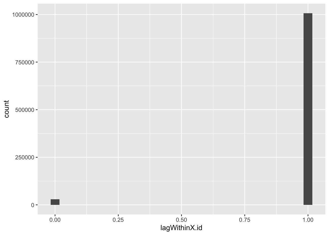

f1_dt[, lagWithinX.id.1 := X.id.2 - shift(X.id.2), keyby = .(X.id.1)]

head(f1_dt[, .(X.id.1, X.id.2, lagWithinX.id.1)])

##    X.id.1 X.id.2 lagWithinX.id.1
## 1:     NA     NA              NA
## 2:     NA     NA              NA
## 3:     NA     NA              NA
## 4:     NA     NA              NA
## 5:     NA     NA              NA
## 6:     NA     NA              NA

summary(f1_dt[, .(X.id.1, X.id.2, lagWithinX.id.1)])

##      X.id.1          X.id.2        lagWithinX.id.1
##  Min.   :  1.0   Min.   :      1   Min.   :0.000  
##  1st Qu.:221.0   1st Qu.: 251860   1st Qu.:1.000  
##  Median :460.0   Median : 503705   Median :1.000  
##  Mean   :446.7   Mean   : 503715   Mean   :0.971  
##  3rd Qu.:672.0   3rd Qu.: 755582   3rd Qu.:1.000  
##  Max.   :895.0   Max.   :1007419   Max.   :1.000  
##  NA's   :11155   NA's   :11155     NA's   :12050

ggplot2::ggplot(f1_dt, aes(x = lagWithinX.id.1)) +
  geom_histogram()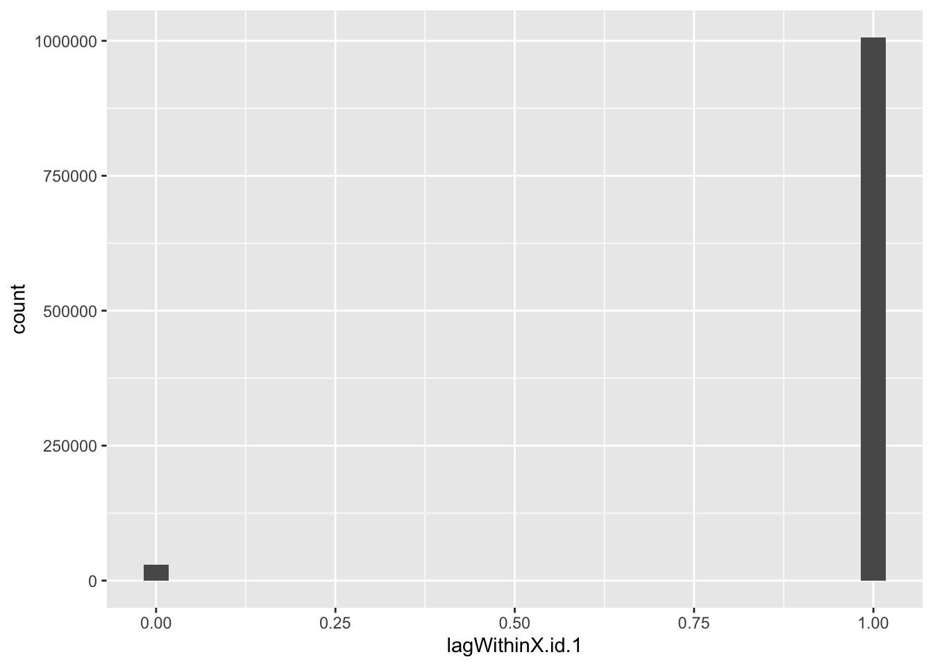

Yep. So we need a way to set the first dateTime within each id and then increase it by 30 minutes each row.

2.6 Setting true dateTime

Based on our hunch…

f1_dt[, counter :=1]
f1_dt[, cumsum := cumsum(counter), keyby = .(X.id.1)] # add up within X.id.1
f1_dt[, dateTime := ba_StartDate] # constant
f1_dt[, dateTime := dateTime + (cumsum * 30 * 60)] # add on the number of seconds since start

f1_dt[, date := lubridate::date(dateTime)]
f1_dt[, month := lubridate::month(dateTime,
                                  label = TRUE, 
                                  abbr = TRUE)
      ]

head(f1_dt[!is.na(X.id.1), .(X.id.1, X.id.2, ba_EndDate, ba_EndTime, 
                             ba_StartDate, dateTime)])

##    X.id.1 X.id.2          ba_EndDate          ba_EndTime        ba_StartDate
## 1:      1      1 2020-01-27 21:25:00 2019-05-12 05:00:00 2018-11-30 11:00:00
## 2:      1      2 2020-01-27 21:25:00 2019-05-12 05:00:00 2018-11-30 11:00:00
## 3:      1      3 2020-01-27 21:25:00 2019-05-12 05:00:00 2018-11-30 11:00:00
## 4:      1      4 2020-01-27 21:25:00 2019-05-12 05:00:00 2018-11-30 11:00:00
## 5:      1      5 2020-01-27 21:25:00 2019-05-12 05:00:00 2018-11-30 11:00:00
## 6:      1      6 2020-01-27 21:25:00 2019-05-12 05:00:00 2018-11-30 11:00:00
##               dateTime
## 1: 2018-11-30 11:30:00
## 2: 2018-11-30 12:00:00
## 3: 2018-11-30 12:30:00
## 4: 2018-11-30 13:00:00
## 5: 2018-11-30 13:30:00
## 6: 2018-11-30 14:00:00

summary(f1_dt[!is.na(X.id.1), .(X.id.1, X.id.2, ba_EndDate, ba_EndTime,
                                ba_StartDate, dateTime)])

##      X.id.1          X.id.2          ba_EndDate                 
##  Min.   :  1.0   Min.   :      1   Min.   :2020-01-27 21:25:00  
##  1st Qu.:221.0   1st Qu.: 251860   1st Qu.:2020-01-27 21:25:00  
##  Median :460.0   Median : 503705   Median :2020-01-27 21:25:00  
##  Mean   :446.7   Mean   : 503715   Mean   :2020-01-27 21:25:00  
##  3rd Qu.:672.0   3rd Qu.: 755582   3rd Qu.:2020-01-27 21:25:00  
##  Max.   :895.0   Max.   :1007419   Max.   :2020-01-27 21:25:00  
##                                                                 
##    ba_EndTime                   ba_StartDate                
##  Min.   :2019-05-12 05:00:00   Min.   :2018-11-30 11:00:00  
##  1st Qu.:2019-05-12 05:00:00   1st Qu.:2018-11-30 11:00:00  
##  Median :2019-05-12 05:00:00   Median :2018-11-30 11:00:00  
##  Mean   :2019-05-12 05:00:00   Mean   :2018-11-30 11:00:00  
##  3rd Qu.:2019-05-12 05:00:00   3rd Qu.:2018-11-30 11:00:00  
##  Max.   :2019-05-12 05:00:00   Max.   :2018-11-30 11:00:00  
##  NA's   :1036567                                            
##     dateTime                  
##  Min.   :2018-11-30 11:30:00  
##  1st Qu.:2018-12-06 19:00:00  
##  Median :2018-12-13 05:30:00  
##  Mean   :2018-12-16 18:50:09  
##  3rd Qu.:2018-12-25 12:30:00  
##  Max.   :2019-01-27 23:30:00  
##

skim(f1_dt[, .(X.id.1, X.id.2,ba_EndDate, ba_EndTime, ba_StartDate, dateTime)])

(#tab:f1_makeDateTime)Data summary

Name	…[]
Number of rows	1048574
Number of columns	6
_______________________
Column type frequency:
numeric	2
POSIXct	4
________________________
Group variables	None

Variable type: numeric

skim_variable	n_missing	complete_rate	mean	sd	p0	p25	p50	p75	p100	hist
X.id.1	11155	0.99	446.71	259.02	1	221.0	460	672.0	895	▇▆▇▆▇
X.id.2	11155	0.99	503715.04	290824.01	1	251860.5	503705	755582.5	1007419	▇▇▇▇▇

Variable type: POSIXct

skim_variable	n_missing	complete_rate	min	max	median	n_unique
ba_EndDate	11155	0.99	2020-01-27 21:25:00	2020-01-27 21:25:00	2020-01-27 21:25:00	1
ba_EndTime	1047722	0.00	2019-05-12 05:00:00	2019-05-12 05:00:00	2019-05-12 05:00:00	1
ba_StartDate	11155	0.99	2018-11-30 11:00:00	2018-11-30 11:00:00	2018-11-30 11:00:00	1
dateTime	11155	0.99	2018-11-30 11:30:00	2019-01-27 23:30:00	2018-12-13 05:30:00	2809

Looks OK: dateTime implies we have 2810 half hours represented which implies we only have 2 months of data.

f1_dt[, .(nObs = .N), keyby = .(month,
                                year = lubridate::year(dateTime))][order(year)]

##    month year   nObs
## 1:   Nov 2018  21925
## 2:   Dec 2018 849112
## 3:   Jan 2019 166382
## 4:  <NA>   NA  11155

Looks like it but this depends if we’ve coded dateTime correctly.

Let’s see how many households (IDs) and observations we have over time.

plotDT <- f1_dt[, .(nX.id = uniqueN(X.id)), keyby = .(date)]
ggplot2::ggplot(plotDT, aes(y = nX.id, x = date)) +
  geom_point()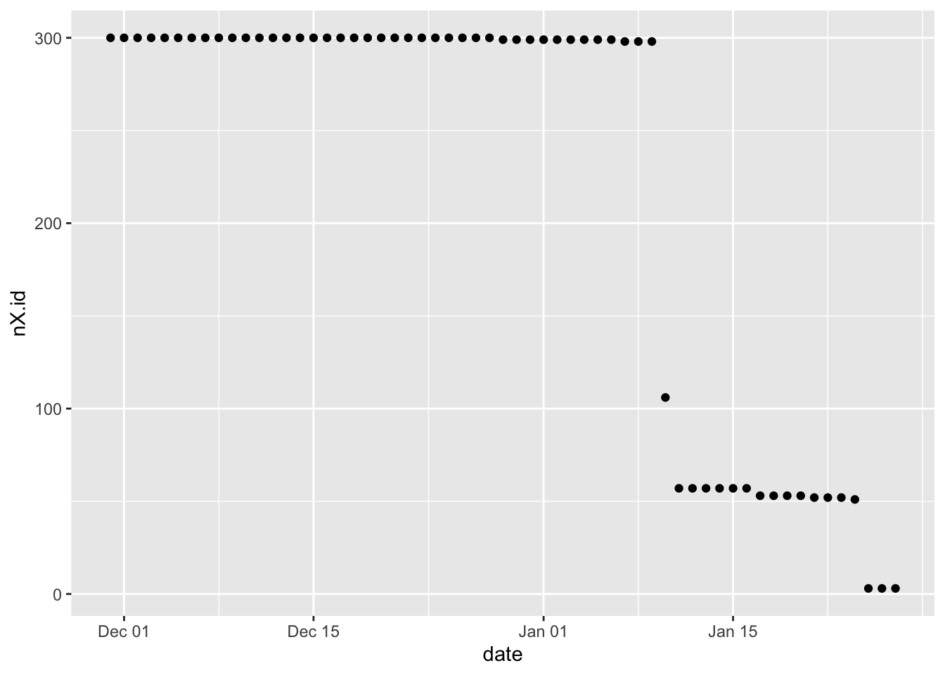

(#fig:plot_f1_NumberOfIXDsByDate)Number of unique X.id by date

plotDT <- f1_dt[, .(nX.id.1 = uniqueN(X.id.1)), keyby = .(date)]
ggplot2::ggplot(plotDT, aes(y = nX.id.1, x = date)) +
  geom_point()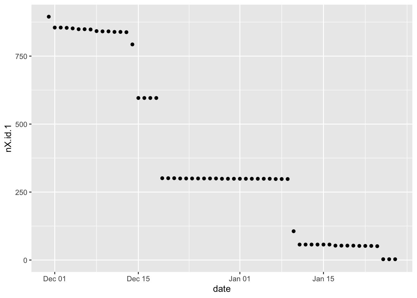

Figure 2.1: Number of unique X.id.1 by date

plotDT <- f1_dt[, .(nObs = .N), keyby = .(date)]
ggplot2::ggplot(plotDT, aes(y = nObs, x = date)) +
  geom_point()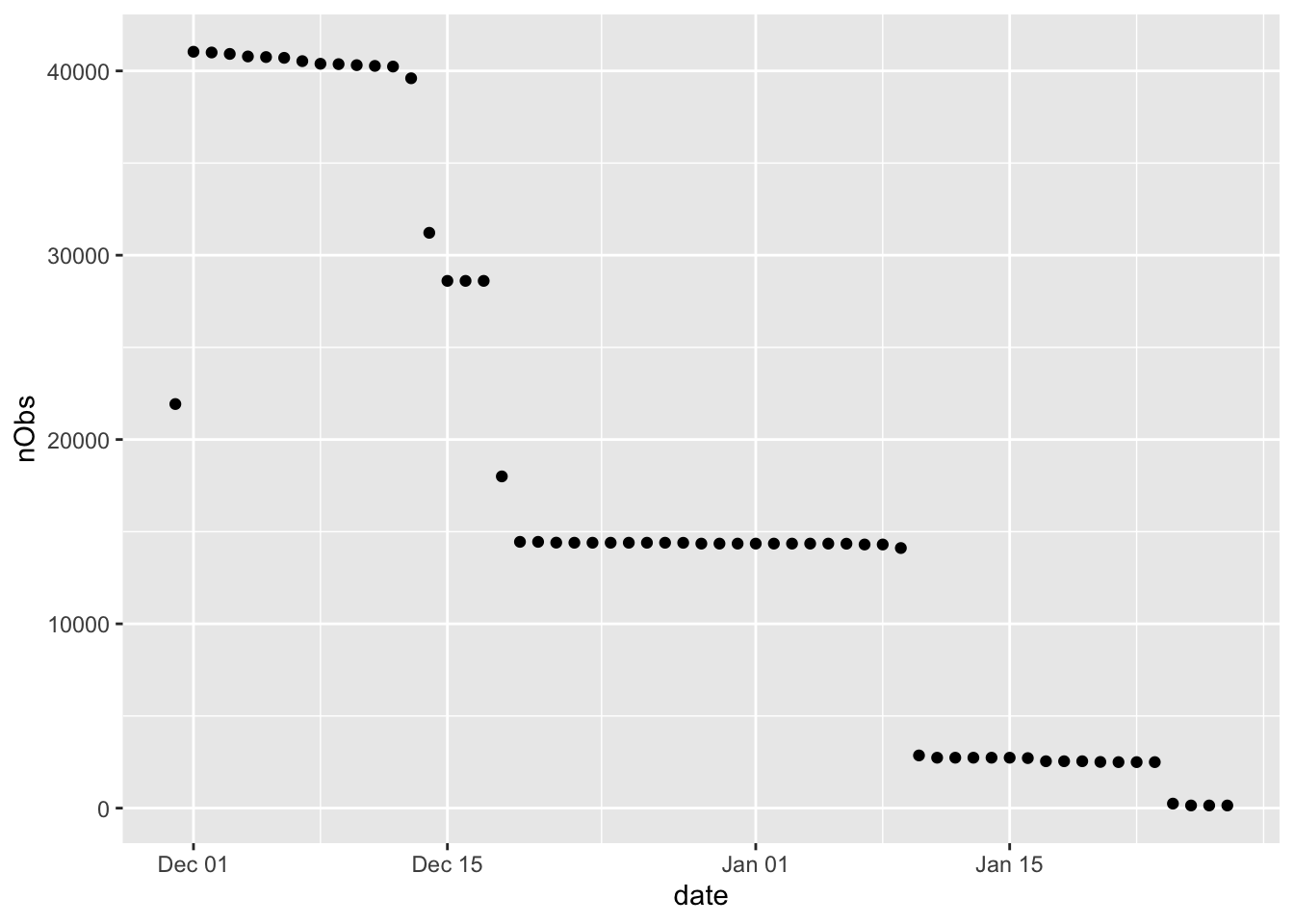

Figure 2.2: Number of obs by date

Yeah. So this does suggest that X.id.2 is a household ID as it follows the pattern of the number of observations (2.1).

2.7 NumberOfReadings

What is this for?

head(f1_dt$NumberOfReadings)

## [1] NA NA NA NA NA NA

ggplot2::ggplot(f1_dt[,.(NumberOfReadings)], aes(x = NumberOfReadings)) +
  geom_histogram()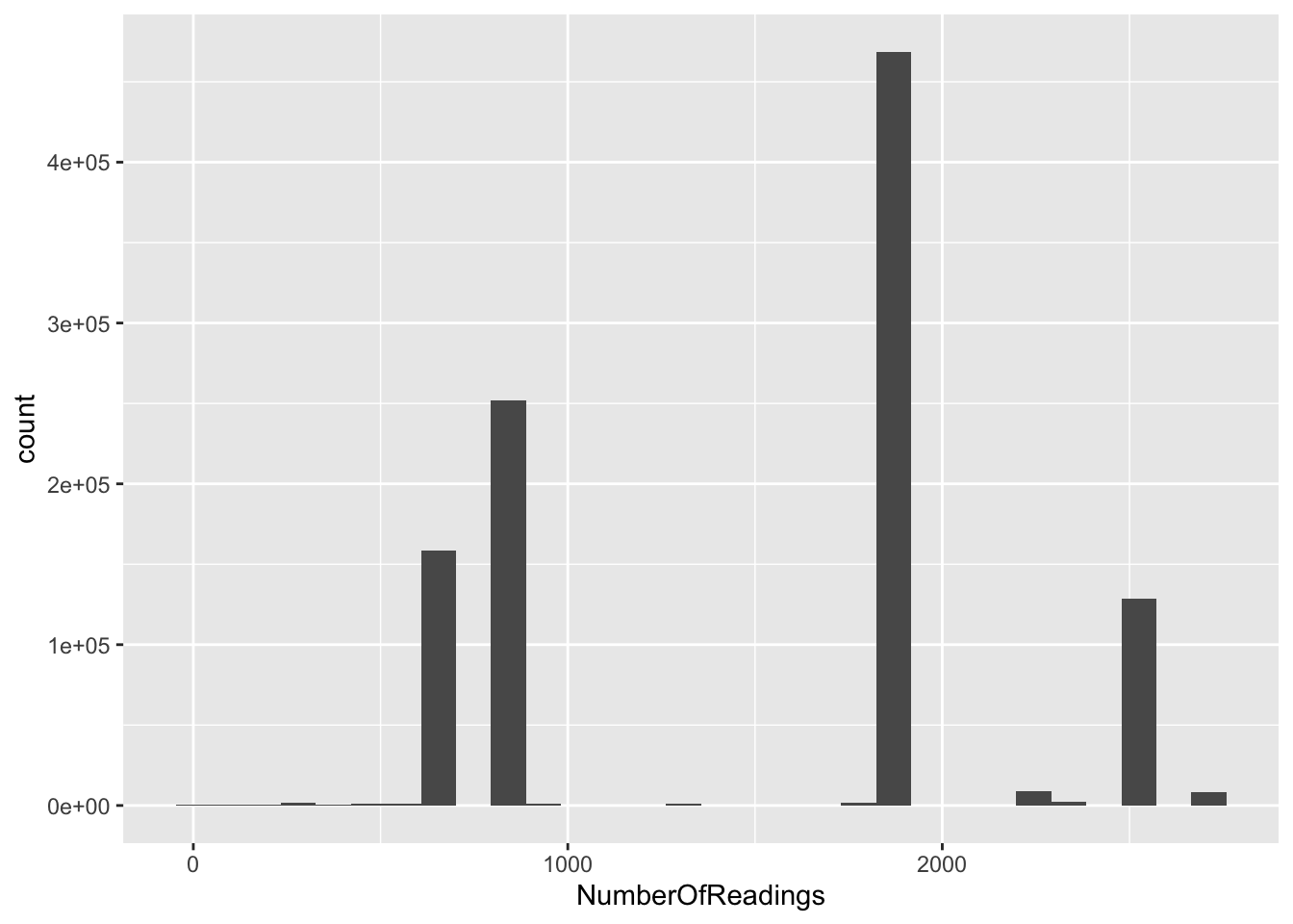

OK, so why do we have some rows with lots of readings and some with far fewer? Is this just meta-data for each id - does it tell us how many readings we have for each ID?

2.8 Value

Value should (ideally) be consumption per half hour.

skim(f1_dt$Value)

Table 2.2: Data summary

Name	f1_dt$Value
Number of rows	1048574
Number of columns	1
_______________________
Column type frequency:
numeric	1
________________________
Group variables	None

Variable type: numeric

skim_variable	n_missing	complete_rate	mean	sd	p0	p25	p50	p75	p100	hist
data	11155	0.99	231.76	32.14	0	234	237	240	917	▁▇▁▁▁

ggplot2::ggplot(f1_dt[,.(Value, NumberOfReadings)], aes(x = NumberOfReadings , y = Value)) +
  geom_point()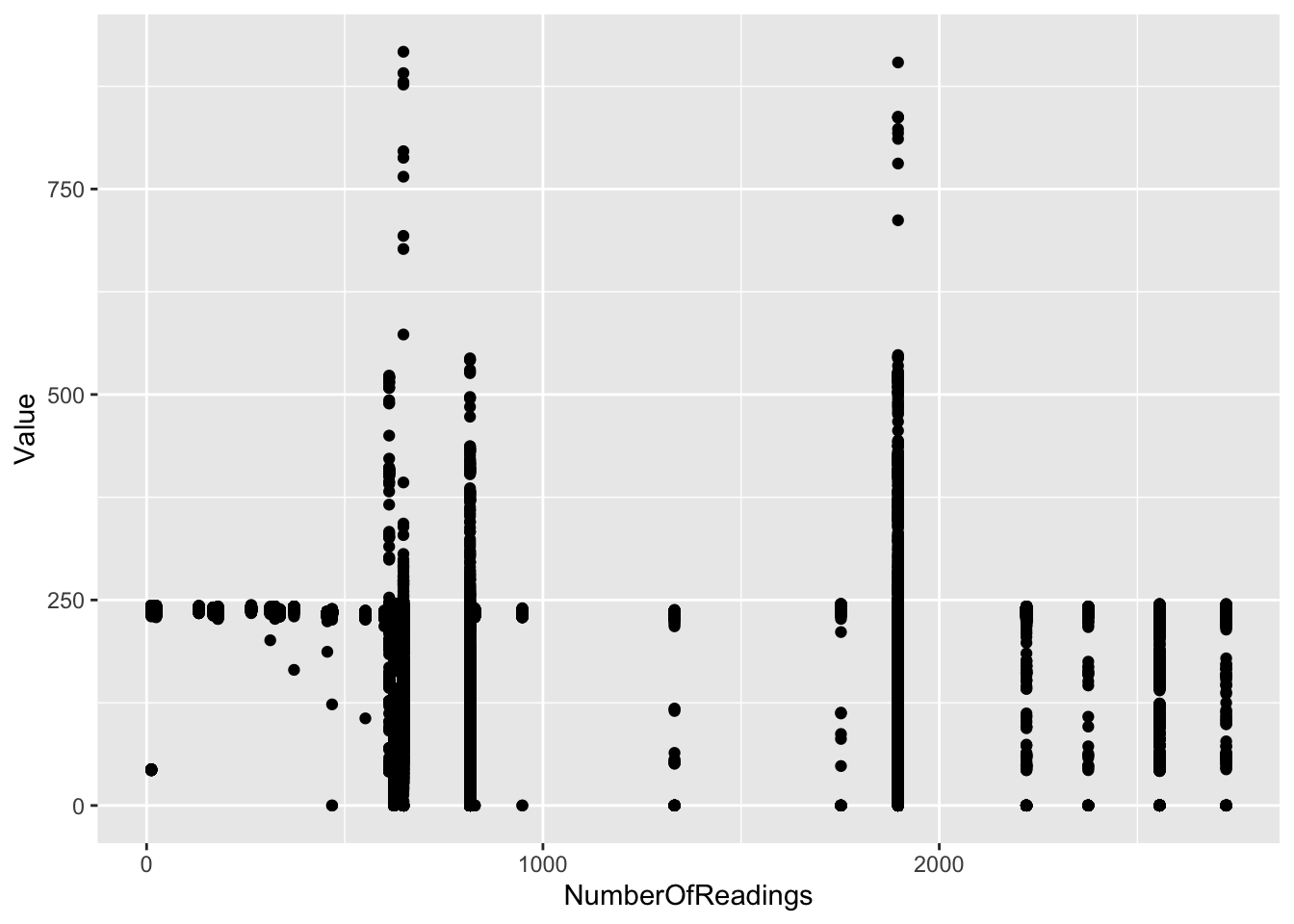

Figure 2.3: Distribution of Value

ggplot2::ggplot(f1_dt[,.(Value, NumberOfReadings)], aes(x = Value)) +
  geom_histogram()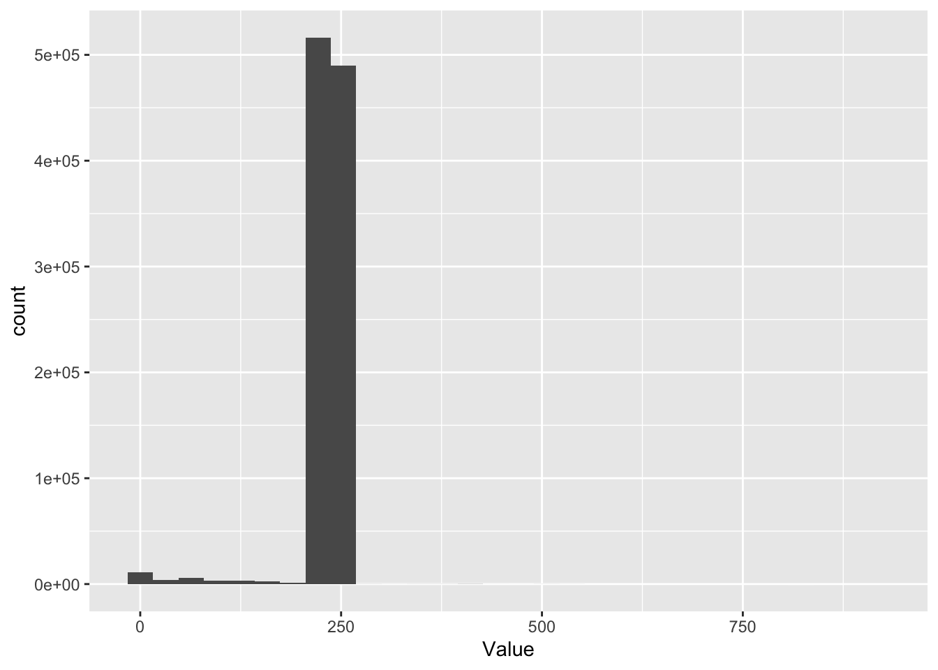

Figure 2.4: Distribution of Value

Well ?? looks a bit odd. Why is there a sort of threshold at 250? We obviously have very few Values over 250…

Try plotting mean of Value by dateTime across all households (remember number of X.id.1s varies across time)

p <- ggplot2::ggplot(f1_dt, aes(x = date , y = Value, group = date)) +
  geom_boxplot()

p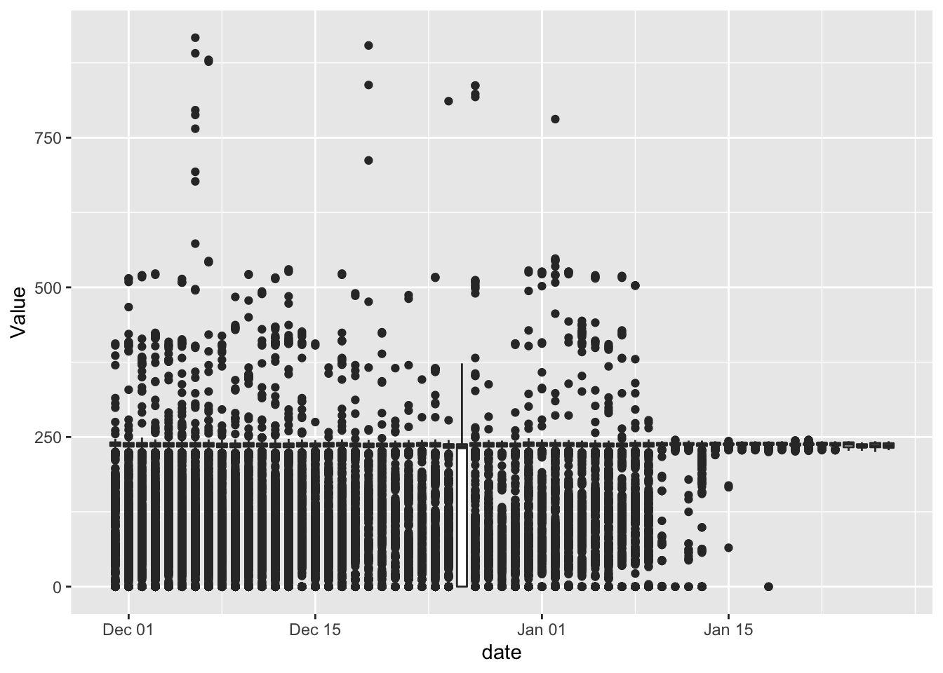

(#fig:plot_f1_valueByDate)Box plot of Value by date

Christmas day looks interesting. But most of the values are below 250 on every other day.

plotDT <- f1_dt[, .(meanValue = mean(Value)), keyby = .(dateTime)]
  ggplot2::ggplot(plotDT, aes(x = dateTime , y = meanValue)) +
  geom_point()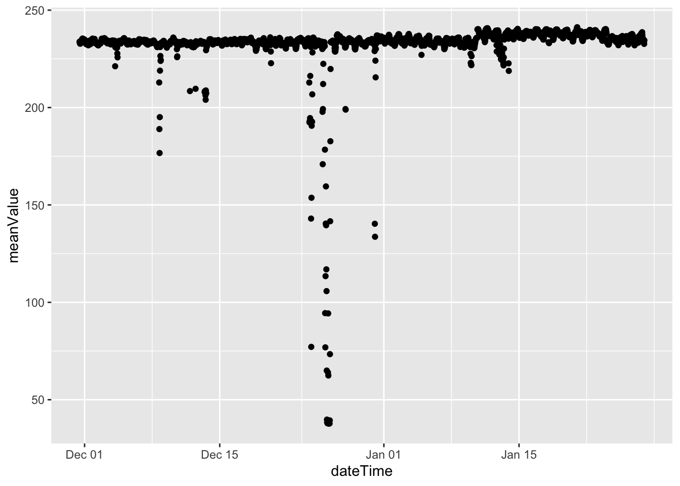

(#fig:plot_f1_valueMeanByDate)Mean Value by date

f1_dt[, hms := hms::as_hms(dateTime)]
f1_dt[, month := lubridate::month(dateTime, label = TRUE, abbr = TRUE)]

ggplot2::ggplot(f1_dt[!is.na(month)], aes(x = hms , y = Value, group = hms)) +
  geom_boxplot() +
  facet_grid(. ~ month)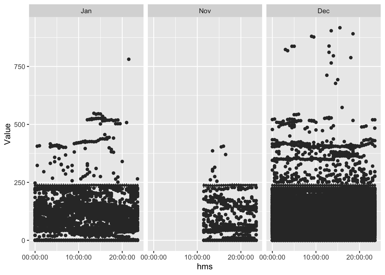

(#fig:plot_f1_valueByTime)Value by time of day

plotDT <- f1_dt[!is.na(month), .(meanValue = mean(Value)), keyby = .(month, hms)]
  
ggplot2::ggplot(plotDT, aes(x = hms , y = meanValue)) +
  geom_point() +
  facet_grid(. ~ month)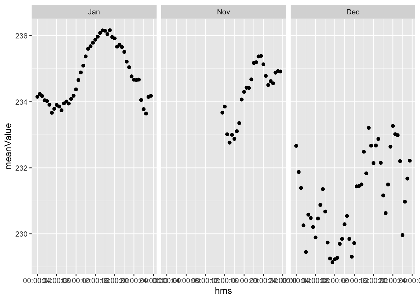

Figure 2.5: Mean Value by time of day

What is this? Is this even the right shape?? 2.5 Could be… but the values are weird.

It can’t be voltage can it (with outliers)?

2.9 Initial dataset summary

We really don’t know what most of these data columns are!

3 Second dataset

Let’s hope this is more heplful!!

4 Runtime

Analysis completed in 321.53 seconds ( 5.36 minutes) using knitr in RStudio with R version 3.6.3 (2020-02-29) running on x86_64-apple-darwin15.6.0.

5 R environment

5.1 R packages used

base R (R Core Team 2016)
bookdown (Xie 2016a)
data.table (Dowle et al. 2015)
ggplot2 (Wickham 2009)
kableExtra (Zhu 2018)
knitr (Xie 2016b)
lubridate (Grolemund and Wickham 2011)
rmarkdown (Allaire et al. 2018)
skimr (Arino de la Rubia et al. 2017)
XML (Lang and CRAN Team 2019)

5.2 Session info

## R version 3.6.3 (2020-02-29)
## Platform: x86_64-apple-darwin15.6.0 (64-bit)
## Running under: macOS Catalina 10.15.3
## 
## Matrix products: default
## BLAS:   /Library/Frameworks/R.framework/Versions/3.6/Resources/lib/libRblas.0.dylib
## LAPACK: /Library/Frameworks/R.framework/Versions/3.6/Resources/lib/libRlapack.dylib
## 
## locale:
## [1] en_NZ.UTF-8/en_NZ.UTF-8/en_NZ.UTF-8/C/en_NZ.UTF-8/en_NZ.UTF-8
## 
## attached base packages:
## [1] stats     graphics  grDevices utils     datasets  methods   base     
## 
## other attached packages:
## [1] XML_3.99-0.3      skimr_2.1         kableExtra_1.1.0  ggplot2_3.3.0    
## [5] hms_0.5.3         lubridate_1.7.4   data.table_1.12.8
## 
## loaded via a namespace (and not attached):
##  [1] tidyselect_1.0.0  xfun_0.12         repr_1.1.0        purrr_0.3.3      
##  [5] colorspace_1.4-1  vctrs_0.2.4       htmltools_0.4.0   viridisLite_0.3.0
##  [9] yaml_2.2.1        base64enc_0.1-3   utf8_1.1.4        rlang_0.4.5      
## [13] R.oo_1.23.0       pillar_1.4.3      glue_1.3.2        withr_2.1.2      
## [17] R.utils_2.9.2     lifecycle_0.2.0   stringr_1.4.0     munsell_0.5.0    
## [21] gtable_0.3.0      rvest_0.3.5       R.methodsS3_1.8.0 evaluate_0.14    
## [25] labeling_0.3      knitr_1.28        fansi_0.4.1       highr_0.8        
## [29] Rcpp_1.0.4        readr_1.3.1       scales_1.1.0      webshot_0.5.2    
## [33] jsonlite_1.6.1    farver_2.0.3      digest_0.6.25     stringi_1.4.6    
## [37] bookdown_0.18     dplyr_0.8.5       grid_3.6.3        cli_2.0.2        
## [41] tools_3.6.3       magrittr_1.5      tibble_2.1.3      crayon_1.3.4     
## [45] tidyr_1.0.2       pkgconfig_2.0.3   xml2_1.2.5        assertthat_0.2.1 
## [49] rmarkdown_2.1     httr_1.4.1        rstudioapi_0.11   R6_2.4.1         
## [53] compiler_3.6.3

References

Allaire, JJ, Yihui Xie, Jonathan McPherson, Javier Luraschi, Kevin Ushey, Aron Atkins, Hadley Wickham, Joe Cheng, and Winston Chang. 2018. Rmarkdown: Dynamic Documents for R. https://CRAN.R-project.org/package=rmarkdown.

Arino de la Rubia, Eduardo, Hao Zhu, Shannon Ellis, Elin Waring, and Michael Quinn. 2017. Skimr: Skimr. https://github.com/ropenscilabs/skimr.

Dowle, M, A Srinivasan, T Short, S Lianoglou with contributions from R Saporta, and E Antonyan. 2015. Data.table: Extension of Data.frame. https://CRAN.R-project.org/package=data.table.

Grolemund, Garrett, and Hadley Wickham. 2011. “Dates and Times Made Easy with lubridate.” Journal of Statistical Software 40 (3): 1–25. http://www.jstatsoft.org/v40/i03/.

Lang, Duncan Temple, and the CRAN Team. 2019. XML: Tools for Parsing and Generating Xml Within R and S-Plus. https://CRAN.R-project.org/package=XML.

R Core Team. 2016. R: A Language and Environment for Statistical Computing. Vienna, Austria: R Foundation for Statistical Computing. https://www.R-project.org/.

Wickham, Hadley. 2009. Ggplot2: Elegant Graphics for Data Analysis. Springer-Verlag New York. http://ggplot2.org.

Xie, Yihui. 2016a. Bookdown: Authoring Books and Technical Documents with R Markdown. Boca Raton, Florida: Chapman; Hall/CRC. https://github.com/rstudio/bookdown.

———. 2016b. Knitr: A General-Purpose Package for Dynamic Report Generation in R. https://CRAN.R-project.org/package=knitr.

Zhu, Hao. 2018. KableExtra: Construct Complex Table with ’Kable’ and Pipe Syntax. https://CRAN.R-project.org/package=kableExtra.

Exploring Tongan Smart Meter Data

Code and notes

Ben Anderson (ben.anderson@otago.ac.nz), Centre for Sustainability, University of Otago

Last run at: 2020-03-25 21:36:12

1 Intro

2 Initial dataset - file: CRF_2020_1_28_4296268_1 - Copy.7z

2.1 StartDate

2.2 EndDate

2.3 EndTime

2.4 NumberOfReadings_1

2.5 X.id* variables

2.5.1 X.id

2.5.2 X.id.1

2.5.3 X.id.2

2.5.4 What the ID?

2.6 Setting true dateTime

2.7 NumberOfReadings

2.8 Value

2.9 Initial dataset summary

3 Second dataset

4 Runtime

5 R environment

5.1 R packages used

5.2 Session info

References