Analysis of electric vehicle usage patterns in New Zealand

Statistical report using Flip The Fleet data

1 Health warning

The analysis reported below is work in progress. Please check with the authors before quoting or re-using (with attribution) results/plots. Reporting interim results without checking can seriously damage your health (and career :-). #YMMV.

2 About

2.1 Citation

• Parker, R., Anderson, B., and Myall, D. (2020) Analysis of electric vehicle usage patterns in New Zealand: Statistical report using Flip The Fleet data. University of Otago: Centre for Sustainability

2.2 License

This work is made available under the Creative Commons Attribution-ShareAlike 4.0 International (CC BY-SA 4.0) License.

This means you are free to:

• Share — copy and redistribute the material in any medium or format
• Adapt — remix, transform, and build upon the material for any purpose, even commercially.

Under the following terms:

• Attribution — You must give appropriate credit, provide a link to the license, and indicate if changes were made. You may do so in any reasonable manner, but not in any way that suggests the licensor endorses you or your use.
• ShareAlike — If you remix, transform, or build upon the material, you must distribute your contributions under the same license as the original.
• No additional restrictions — You may not apply legal terms or technological measures that legally restrict others from doing anything the license permits.

Notices:

• You do not have to comply with the license for elements of the material in the public domain or where your use is permitted by an applicable exception or limitation.
• No warranties are given. The license may not give you all of the permissions necessary for your intended use. For example, other rights such as publicity, privacy, or moral rights may limit how you use the material. #YMMV

For the avoidance of doubt and explanation of terms please refer to the full license notice and legal code.

3 Introduction

The New Zealand government has set a target of increasing the number of electric vehicles (EVs) in New Zealand to 64,000 by 2021 (Transpower New Zealand 2017). High penetration of EVs would cause EV recharging to contribute a substantial portion of total electricity load. A report prepared for lines companies Orion, Powerco and Unison by Concept Consulting Group entitled “Driving change - Issues and options to maximise the opportunities from large-scale electric vehicle uptake in New Zealand” predicts that if all current light private vehicles were electric, annual residential electricity consumption would increase by approximately 30%, whereas if all vehicles including trucks were electric, this would increase the total electricity consumption of New Zealand by approximately 41% (Concept Consulting 2018).

New Zealand’s total electricity demand varies throughout the day, with weekdays in particular having two distinct “peaks”; one in the morning, and one in the evening (Transpower New Zealand 2015). Providing the electricity to meet these demand peaks is a costly and inefficient process (Khan, Jack, and Stephenson 2018). Concurrent electric vehicle charging, especially in the early evening when many motorists return home (Speidel and Bräunl 2014; Langbroek, Franklin, and Susilo 2017), would have the potential to negatively impact the operation of the grid through drastically increasing peak loads (Azadfar, Sreeram, and Harries 2015; Langbroek, Franklin, and Susilo 2017), leading to an increased cost of electricity due to the requirement of expensive upgrades to the electricity grid (Stephenson et al. 2017).

The Concept Consulting report considers different methods of EV charging in its models. The assumption that most drivers would begin charging immediately after returning home is referred to as “passive” charging, while charging that is programmed (either by the driver or by an external entity) to occur during off-peak periods is referred to as “smart”. The modelling undertaken in the Concept Consulting report suggests that under a scenario whereby 57% of the current private vehicle fleet were EVs (corresponding to one EV per household), passive charging would cause an increase of peak electricity demand of approximately 3,000MW, whereas if all were charged in a “smart” fashion, there would be no increase in peak demand.

This report extends the work done by Concept Consulting, but utilises actual data collected from electric vehicles, as opposed to using models based on the current New Zealand transport sector. The intention of the report is to provide further insight into the potential effects on the New Zealand electricity grid that may occur with a dramatic increase in EVs, so that these may be planned for and mitigated. It is also inspired by the UK Department of Transport 2018 statistical report (Eyers 2018).

4 Data

Data file used in this report: EVBB_processed_all_v2.0_20190604.csv

4.1 Background

The data used has been provided by ‘Flip the Fleet’, a community organisation that hopes to increase uptake of electric vehicles in New Zealand. Flip the Fleet have been collecting data on electric vehicle usage patterns, via Exact IOT Limited’s blackbox recorder, a small electronic device that connects to the vehicle’s internal computer and sends detailed data about the battery health, power demand, charging rate, speed and other performance information to a secure database.

The subset of this data provided to the University of Otago was collected from 52 domestic electric vehicles monitored from Inf to -Inf. The data consisted of 1,882,040 1 minute interval observations of timestamped odometer readings (in km) together with measurements of charging power (kW) and battery charge state (% charged) linked by a unique anonymised vehicle identifier. The data received contained all available observations but charging was set to 0 kW if the vehicle was non-stationary (speed > 0 km/h) prior to data delivery to the University. This enabled us to automatically exclude charging through regenerative braking from the analysis.

There are a number of important limitations to this data:

• observations were only collected when the car was switched on and/or plugged in and charging. As a result no observations exist for periods when the EV is switched off and so there are large non-erroneous ‘gaps’ in the data which represent ‘no charging’ but which are not included as ‘0 power demand’ in the analyses since to do so would require imputation of a very large number of missing time-stamps for each vehicle. This means we are only able to analyse power demand profiles for vehicles that were known to be charging, not for all vehicles in all time periods;
• data upload relied on mobile 3G data signal and the extent to which gaps in the data are due to data upload errors rather than the vehicle being switched off (as above) is currently unclear;
• these vehicles are driven by ‘early adopters’ who have opted to install the measuring devices in order to collect their vehicle usage data. As a result the data may not be representative of the usage patterns of current or future EV drivers (Rezvani, Jansson, and Bodin 2015; Li et al. 2017).

Even though the use of an anonymised vehicle identifier should prevent the identification of the vehicles in the sample, the fine-grained temporal nature of the data and the relatively small population of EV owners from whom the sample is drawn (Flip The Fleet members) means that the data cannot be publicly released.

4.2 Initial data cleaning

The original supplied data consisted of 1,882,040 observations for 52 EVs for the period 2018-04-05 to 2019-03-01.

Table 4.1: Summary of original data

	id	charge_power_kw	state_of_charge_percent	odometer_km	r_dateTime	dvID	timeChr
	Length:1882040	Min. : 0.00	Min. : 0.00	Min. :-62920	Min. :2018-04-05 10:34:41	Length:1882040	Length:1882040
	Class :character	1st Qu.: 0.00	1st Qu.: 56.31	1st Qu.: 2166	1st Qu.:2018-10-12 13:27:42	Class :character	Class1:hms
	Mode :character	Median : 1.30	Median : 70.41	Median : 5309	Median :2018-11-25 21:21:08	Mode :character	Class2:difftime
	NA	Mean : 1.59	Mean : 69.00	Mean : 7790	Mean :2018-11-22 14:22:36	NA	Mode :numeric
	NA	3rd Qu.: 1.85	3rd Qu.: 83.05	3rd Qu.: 11154	3rd Qu.:2019-01-13 22:10:02	NA	NA
	NA	Max. :74940.42	Max. :1677.72	Max. : 73607	Max. :2019-03-01 17:42:35	NA	NA
	NA	NA	NA	NA’s :1255614	NA’s :137	NA	NA

Table 4.2 reports the raw charging data values and illustrates the presence of both 0 values and some very large values.

Table 4.2: Descriptive statistics for charging (kW, raw data)

Year	Month	Mean kW	Median kW	Min kW	Max kW	n Obs	n EVs
2018	Apr	23.37	0.00	0	74940.42	5904	2
2018	May	19.52	0.00	0	12044.16	13191	7
2018	Jun	0.76	0.00	0	30.76	22468	10
2018	Jul	1.28	0.00	0	266.26	60776	13
2018	Aug	1.33	0.00	0	48.26	77577	14
2018	Sep	1.69	1.41	0	49.35	178884	37
2018	Oct	1.55	1.43	0	57.91	309239	43
2018	Nov	1.60	1.48	0	70.16	332960	44
2018	Dec	1.55	1.49	0	49.21	299216	42
2019	Jan	0.90	0.00	0	49.40	291236	42
2019	Feb	1.24	1.23	0	49.50	285737	40
2019	Mar	1.64	1.65	0	6.33	4715	32

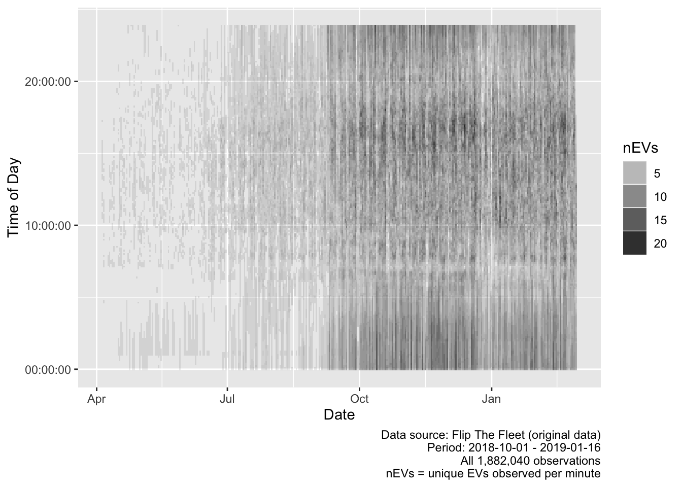
Figure 4.1: Number of unique EVs observed by time of day and date

Figure 4.1 shows the number of unique EVs observed by time of day and date. As we can see the early part of the sample is sparse and indeed the maximum number of EVs observed in any 15 minute time period was only 21 out of a possible total of 52. While this will not affect some analyses, it is likely to introduce error and small sample effects to summary analyses (e.g. means) or month by month analyses. In some sections the analysis will therefore be restricted to the data from September to January.

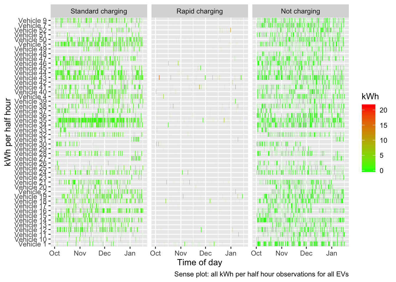
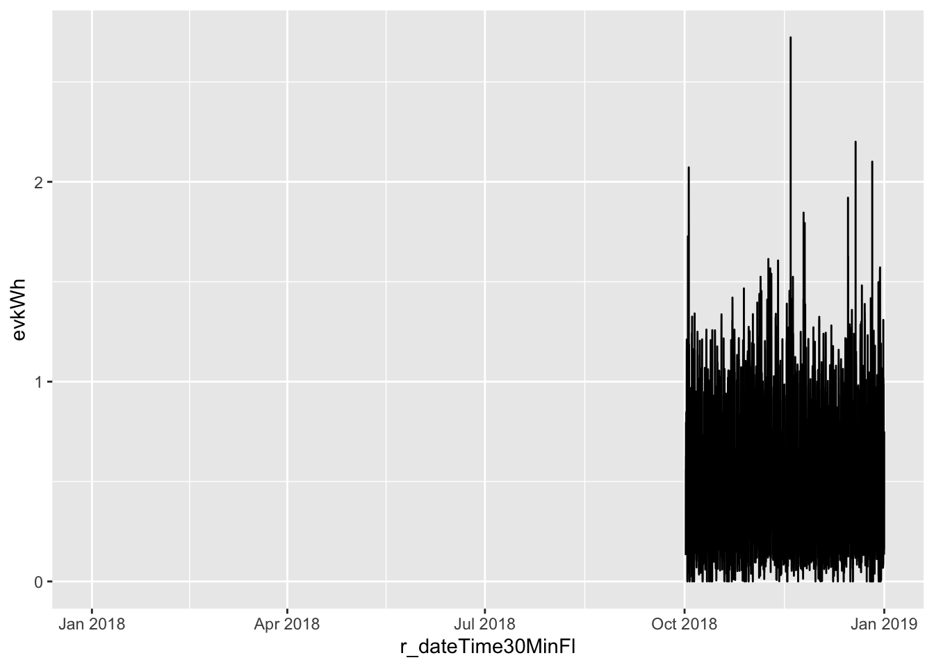
Figure 4.2 plots the number of observations per half hour by EV for the raw data. It appears to suggest that there is a large gap in the charging observations in February. This is not easily explainable as non-charging (i.e. driving) observations continue through this period.

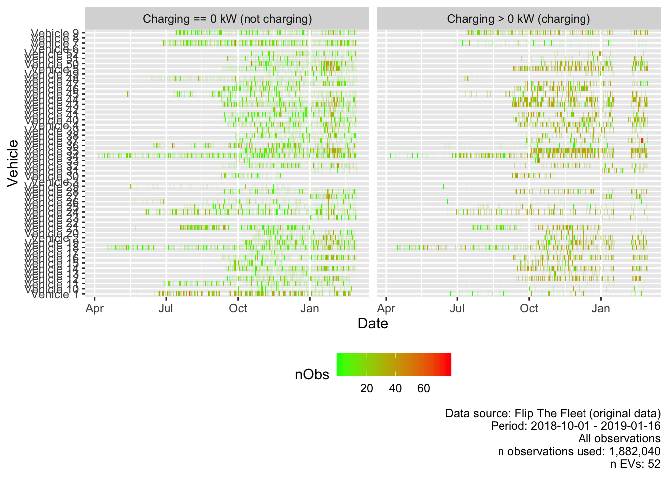
Figure 4.2: Observed charging (raw data)

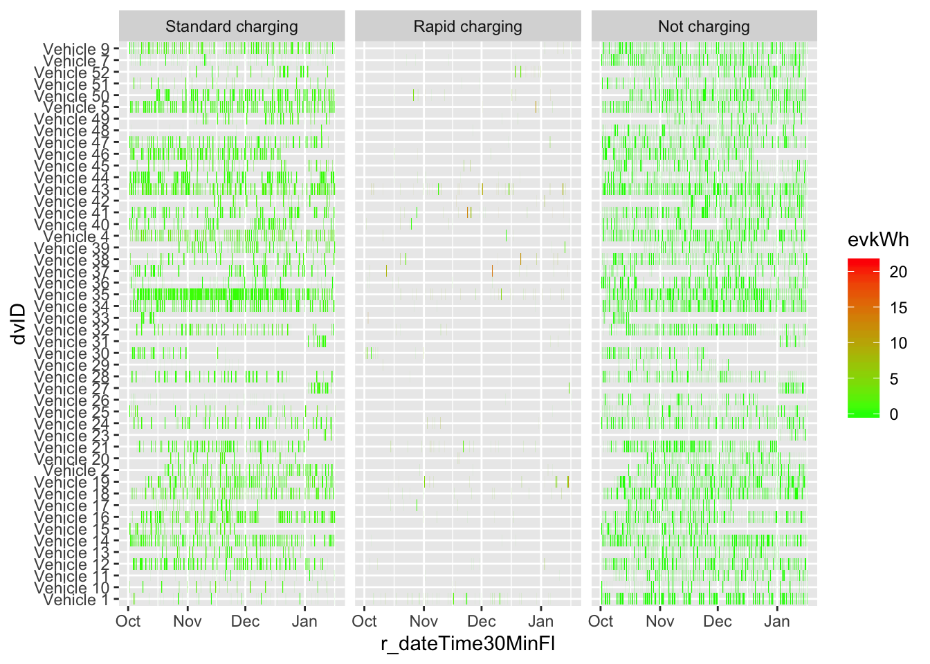
Figure 4.3 shows the unique number of EVs recorded on each day by whether or not they were charging and reflects the period over which Flip The Fleet installed the data collection boxes. It also shows the unexplained drop in charging observations during February.

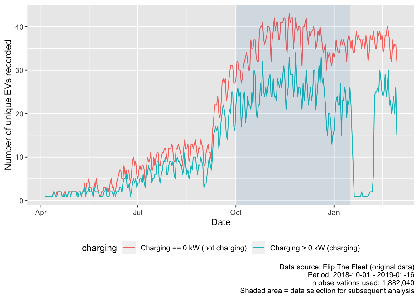
Figure 4.3: Number of unique EVs observed by time of day and date

Finally, 4.3 shows that a small number of EVs have very few observations, in some cases not extending beyond 1 day (shown as 0 days observed).

Table 4.3: Number of observations and start/end dates for vehicles (6 most scarce)

id	nObs	startTime	endTime	meankWCharging	maxkWCharging	nDaysObserved
0cc746a3f5ae75ee94068a8354b6be08	3	2018-09-09 10:46:30	2018-09-09 10:48:42	0.000	0.000	0 days
01583b8a5f0344cc4aa3b3939a27af2a	4	2018-09-09 10:34:12	2018-09-09 10:36:25	0.000	0.000	0 days
4a6bb6e7ffc28d9d8eda7b4c6377a027	19	2018-09-08 08:48:38	2018-09-09 10:27:50	4.225	27.557	1 days
126c8759ec95ba40070b16a11fe0e587	258	2018-09-30 11:54:18	2018-09-30 19:24:05	1.587	1.960	1 days
6e3293c77f562262ed6608db1b596d36	4315	2018-05-15 14:48:15	2018-12-06 13:25:56	0.287	47.246	205 days
781f06f7d7bb80b74c399326be0d3e28	5469	2018-09-28 11:25:58	2018-10-15 16:21:57	2.369	47.687	18 days

Taking all of the above into account we have therefore discarded:

• the 5 vehicles that had no recorded charging observations (this also discarded those with very few observations - see Table 4.3);
• 45 instances of charging power greater than 120kW. These were considered anomalies and as these exceed the capacity of the highest charging stations currently available in New Zealand (Concept Consulting 2018);
• 61 instances of battery state of charge observations of greater than 100%;
• all observations collected before 2018-10-01 and after 2019-01-16 in order to focus analysis on the periods with most EVs present in the data and avoid periods of apparently systematic missing data. It is hoped that this will reduce the extent to which the charging behaviour of a small number of EV owners will skew the aggregated results.

This left 48 remaining vehicles, and 1,074,730 observations as shown in Table 4.4.

Table 4.4: Descriptive statistics for charging (kW, clean data)

Year	Month	Mean kW	Median kW	Min kW	Max kW	n Obs	n EVs
2018	Oct	1.55	1.43	0	57.91	304777	43
2018	Nov	1.60	1.48	0	70.16	332960	44
2018	Dec	1.55	1.49	0	49.21	299216	42
2019	Jan	1.75	1.53	0	49.40	137777	42

4.3 Definitions and preparation

4.3.1 Charge type

Charging data has been broadly separated into two separate categories, ‘Standard’ and ‘Rapid’. Standard charging is defined to be when the charger is reading less than or equal to 7.4 kW - this is considered the upper limit of ordinary home charging without an expensive wiring upgrade (Concept Consulting 2018). Rapid charging is defined as all charging greater than 7.4 kW, and would probably occur at designated and purpose-built public charging stations.

It should be noted that this method is not always accurate since we can identify apparent sequences of charging which start at > 7.4 kW and decline to < 7.4 kW over a relatively short period or vice versa (see Section 8.3.1). In this circumstance the first observation will be correctly classified as ‘Rapid’ but the lower observations, which we assume are lower power ‘top-ups’ at the end of a rapid charge will be incorrectly classified as ‘Standard’. As an example, we know that there are 86 sequences of charging events (out of a total of 13798) where the first and last charge types do not match.

This is clarified and corrected in Section 4.3.2 for charging begin/end pairs (and thus in the results that use this data) but has yet to be resolved in other sections which use all charging observations. As a result we may currently be under-estimating the number of rapid charge observations and over-estimating the mean power demand of standard charges where we conduct analysis using all charging observations.

Figure 4.4 shows the distribution of observed charging kW demand by inferred charge type without correcting for potential mis-classifications. Setting aside the small number of potential misclassifications noted above, the plot confirms the validity of our definition and shows that rapid charges were relatively rare in the dataset. rapid charges have two distinct power demand ‘peaks’ at ~22kW and ~45kW while the far more common standard charging was mostly concentrated around 1.8kW and 3kW, with a smaller concentration around 6kW.

Table 4.5: Descriptive statistics for charging (kW) by inferred charge type

chargeType	Mean kW	Median kW	Min kW	Max kW
Standard charging	2.09	1.76	0.5	7.40
Rapid charging	30.76	31.09	7.4	70.16
Not charging	0.00	0.00	0.0	0.00

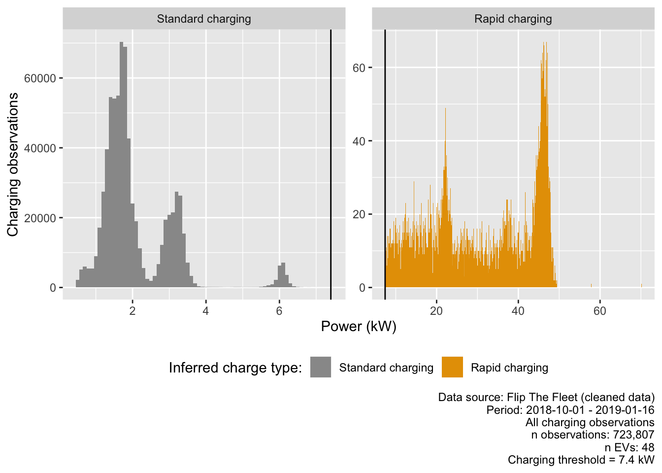
Figure 4.4: Observed power demand distribution by charge type where charging observed (standard vs rapid threshold shown as dark vertical line)

Finally, we test the temporal distribution of observed charging by aggregating to half-hours. Figure 4.5 gives some indication of the relative prevalence of each charging type.

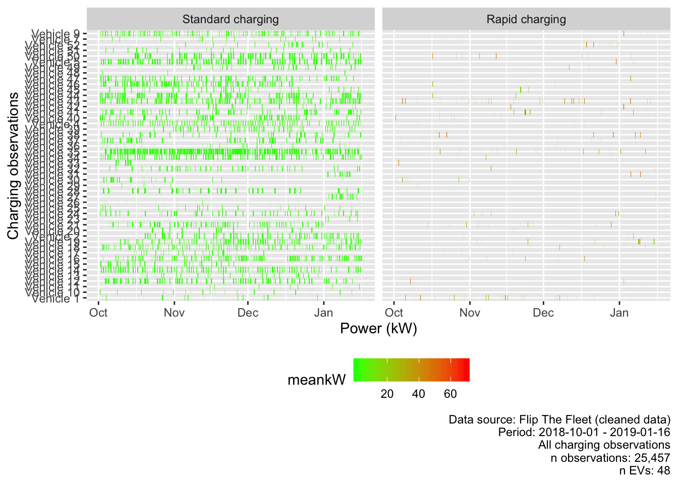
Figure 4.5: Observed charging

4.3.2 Charge sequences

In order to determine charging durations, we have identified and extracted observations which are the start and end of charging sequences. This is done using the following logic:

• rows were coded as “charging begins” if the charging power was greater than zero and the previous and following row’s charging power were (respectively) equal to zero and greater than zero;
• rows were coded as “charge ends” if the charging power was greater than zero and the previous and following row’s charging power were (respectively) greater than zero and equal to zero;
• rows were coded as “charge in a sequence” if charging power > 0 and the observations either side were also > 0
• rows were coded as “single charge events” if charging power > 0 but the observations either side were 0.

Table 4.6: Charge sequence coding results (all cleaned data)

	Standard charging	Rapid charging	Not charging	NA	Sum
Charging in a seq	699162	6093	0	0	705255
First charge obs in a seq	6519	381	0	0	6900
Last charge in a seq	6575	323	0	0	6898
Not charging (0 kW)	0	0	350923	0	350923
Single charge observation	4650	102	0	0	4752
NA	1	1	0	0	2
Sum	716907	6900	350923	0	1074730

Table 4.6 shows the results of this coding for all clean observations within the selected dates (2018-10-01 - 2019-01-16). As we can see most observations were coded using this scheme and we obtained 6,900 instances of charging starting, and 6,898 instances of charge ending. The additional -2 instances of charge ending than there are of the charge beginning may be due to the first (or last) instance of data collection occurring during mid-charge for some vehicles.

An alternative classification method, tested in Section 8.3.1, added a 120 second maximim threshold to sequences of observations but was not used as it failed to identify sparse sequences of charging events.

Comparison of the begining and end charge types showed, as suspected, that a number of pairs had mis-matching charge-types (see Table 4.7). In all cases charge type was set to ‘Rapid’ if either of the start or end observations was classified as ‘Rapid’. However this correction has only been made with the extracted pairs data and how not yet been applied to the full ‘all observations’ data.

Table 4.7: Charge type errors detected via mis-matching start and end observations vs uncorrected charge type

	Standard charging	Rapid charging	Not charging	Sum
Error: first = Rapid, last = Standard	0	72	0	72
Error: first = Standard, last = Rapid	14	0	0	14
OK: first = Rapid, last = Rapid	0	309	0	309
OK: first = Standard, last = Standard	6505	0	0	6505
Sum	6519	381	0	6900

The charge duration was then calculated as being the time duration between each pair of ‘first in charge sequence’ and ‘last in charge sequence’ observations.

Figure 4.6 shows the overall distribution of all charging sequences using the corrected charge type. Clearly there are very small and a few very large values for both charging types.

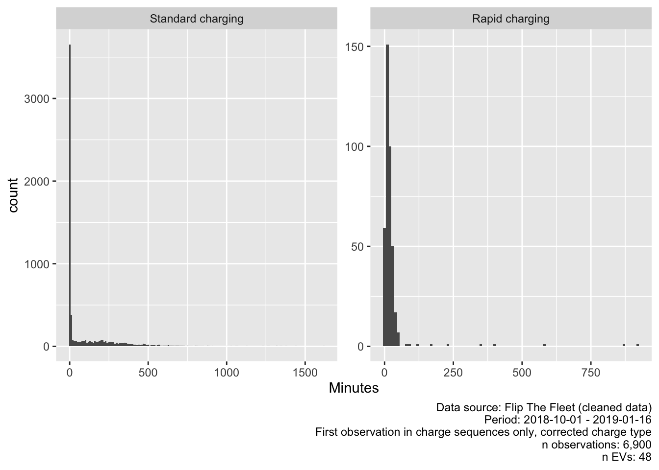
Figure 4.6: Duration of charging sequences by corrected charge type

Table 4.8 shows the overall distributions and indicates the extent to which the means are skewed by the very small and a few very large values shown in Figure 4.6.

Table 4.8: Duration of all charge sequences by charge type

chargeTypeCorrected	N	mean	median	min	max
Standard charging	6501	98.25 mins	3.38 mins	0.27 mins	1616.72 mins
Rapid charging	394	25.12 mins	14.28 mins	0.02 mins	922.03 mins

Table 4.9 shows the longest duration ‘standard’ charge events while Table 4.10 shows the longest duration ‘Rapid’ charge events.

Table 4.9: Duration of longest charge sequences (Standard charging)

dvID	startTime	day_of_week	chargeType	chargeTypeCorrected	pairDuration	duration_hours
Vehicle 39	2019-01-04 10:03:05	Fri	Standard charging	Standard charging	1616.72 mins	26.95
Vehicle 28	2018-10-08 13:54:06	Mon	Standard charging	Standard charging	1442.30 mins	24.04
Vehicle 39	2019-01-01 15:39:53	Tue	Standard charging	Standard charging	1380.53 mins	23.01
Vehicle 34	2018-12-08 22:28:58	Sat	Standard charging	Standard charging	1353.40 mins	22.56
Vehicle 39	2018-12-21 17:40:33	Fri	Standard charging	Standard charging	1341.80 mins	22.36
Vehicle 39	2018-11-25 10:44:13	Sun	Standard charging	Standard charging	1324.10 mins	22.07
Vehicle 35	2019-01-05 16:58:43	Sat	Standard charging	Standard charging	1315.95 mins	21.93
Vehicle 9	2019-01-01 03:35:49	Tue	Standard charging	Standard charging	1266.52 mins	21.11
Vehicle 39	2018-12-06 16:54:34	Thu	Standard charging	Standard charging	1264.10 mins	21.07
Vehicle 18	2018-11-22 13:37:53	Thu	Standard charging	Standard charging	1228.23 mins	20.47

Table 4.10: Duration of longest charge sequences (Rapid charging)

dvID	startTime	day_of_week	chargeType	chargeTypeCorrected	pairDuration	duration_hours
Vehicle 43	2019-01-12 09:51:43	Sat	Rapid charging	Rapid charging	922.03 mins	15.37
Vehicle 36	2018-12-05 17:10:19	Wed	Standard charging	Rapid charging	865.70 mins	14.43
Vehicle 12	2018-11-29 21:08:02	Thu	Rapid charging	Rapid charging	582.53 mins	9.71
Vehicle 40	2018-11-15 12:37:03	Thu	Rapid charging	Rapid charging	398.27 mins	6.64
Vehicle 40	2019-01-15 10:39:13	Tue	Rapid charging	Rapid charging	346.25 mins	5.77
Vehicle 43	2018-12-11 15:39:24	Tue	Rapid charging	Rapid charging	227.85 mins	3.80
Vehicle 1	2018-12-06 07:20:46	Thu	Rapid charging	Rapid charging	173.58 mins	2.89
Vehicle 49	2018-12-11 12:40:40	Tue	Rapid charging	Rapid charging	116.37 mins	1.94
Vehicle 21	2018-12-09 20:04:03	Sun	Rapid charging	Rapid charging	90.57 mins	1.51
Vehicle 44	2018-11-19 16:02:37	Mon	Standard charging	Rapid charging	80.27 mins	1.34

Figure 4.7 shows the distribution of very short charging sequences. As we can see these appear to be generally less than 8 minutes in length for Standard Charges.

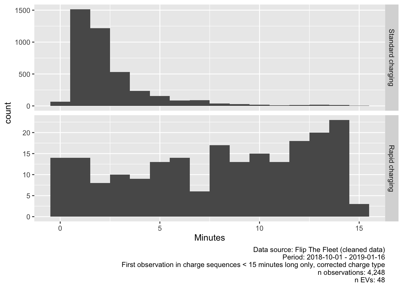
Figure 4.7: Duration of charging sequences < 15 minutes

Manual inspection of the data showed that these short-duration ‘standard’ charging events generally occurred near the end of a longer-duration charging sequence. It appeared that once the vehicle had reached its highest state of charge, charging would intermittently stop and start again. This is probably due to the behaviour of the charger once the battery was almost full.

Table 4.11 repeats the same descriptive statistics reported in Table 4.8 but for all sequences of greater than 8 minute duration. We can now see that the mean and median durations for both Standard and Rapid Charge sequences are closer.

Table 4.11: Duration of charge sequences > 8 minutes by charge type (minutes)

chargeTypeCorrected	N	mean	median	min	max
Standard charging	2594	243.01 mins	207.12 mins	8.03 mins	1616.72 mins
Rapid charging	296	32.18 mins	17.74 mins	8.12 mins	922.03 mins

In addition to the many ‘short’ charging duration values, a small number of unreasonably long charging durations (longer than 14 hours for rapid charging - see Table 4.10) were calculated. As these exceeded the expected charge durations of even the highest capacity vehicles currently available, they were also assumed to be anomalies. The analyses in Section 5.2 below was therefore made with the following charge events excluded from the data:

• duration < 8 minutes for standard charging (3907 observations - noting that some of these may be short low power ‘Rapid charge’ events as discussed in Section 4.3.1)
• duration > 840 minutes (14 hours) for rapid charging (2 observations)

Figure 4.8 shows the distribution of charging sequences with the excessively long or short events removed. These charging durations appear more reasonable when considering standard battery capacities and available charge power.

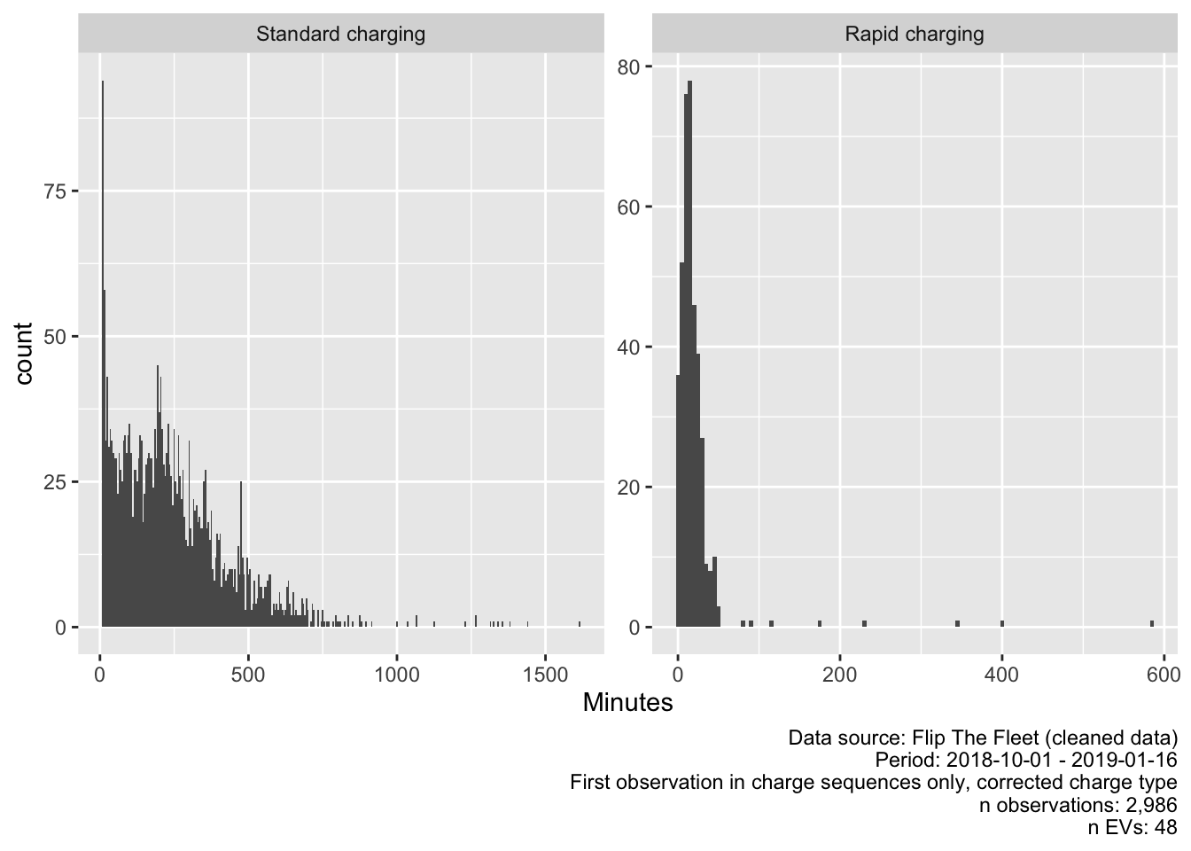
Figure 4.8: Duration of charging sequences with unreasonably long or short values removed

Table 4.12: Duration of charge sequences, final duration data

chargeTypeCorrected	N	mean	median	min	max
Standard charging	2594	243.01 mins	207.12 mins	8.03 mins	1616.72 mins
Rapid charging	392	20.69 mins	14.26 mins	0.02 mins	582.53 mins

5 Results

5.1 Time of charging

It has been suggested that EV charging is more likely to occur in the early evening when drivers return from daily commutes or school pick-ups (Langbroek, Franklin, and Susilo 2017).

Figure 5.1 plots the distribution of each charge type over time of day and confirms the very low incidence of rapid charging. It also supports the suggestion that standard charging (at home) does not appear to begin until later in the evening. Figure 5.2 shows the same results but using a log10 transform of the y axis so that the temporal patterns of the (very few) rapid charging events is visible.

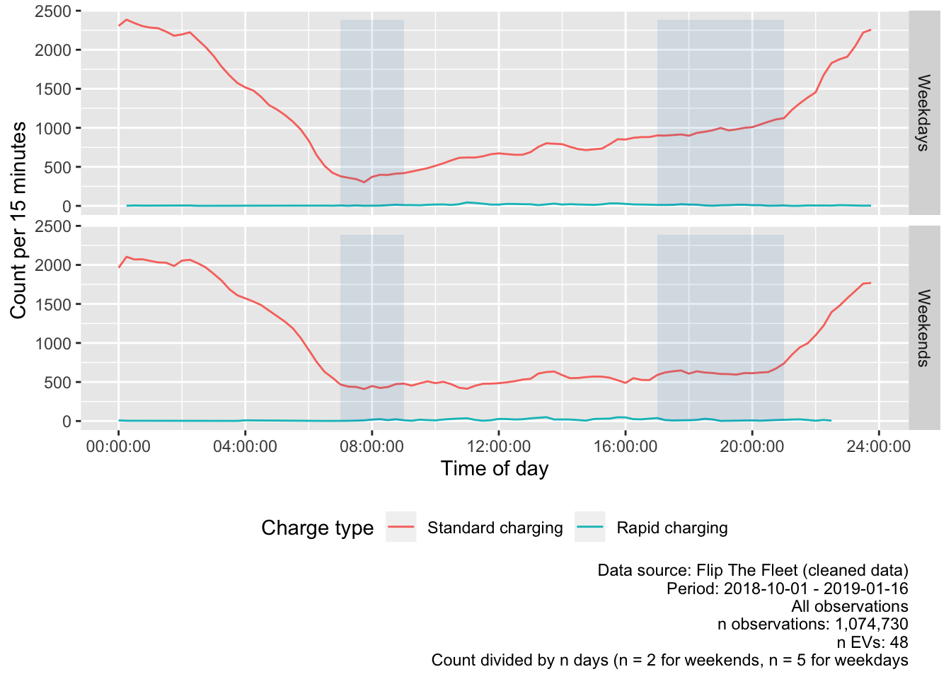
Figure 5.1: Frequency plot of charging start times during weekdays

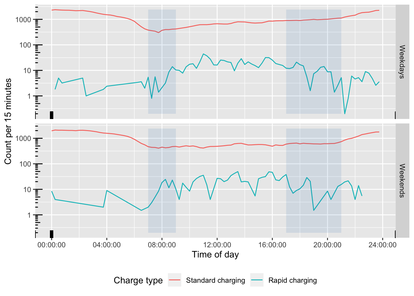
Figure 5.2: log(Frequency) plot of charging start times during weekdays

Figure 5.3 extends this analysis by showing charging and non-charging observations at different times of day by weekday vs weekends using a density plot to show relative distributions over time within each type. The plot clearly shows non-charging during day-time use and also shows a bi-model distribution for rapid charging (non-corrected categorisation). Standard charging also shows a bi-modal distribution with a peak around 22:00 on weekdays and another at 01:00 presumably indicating the use of timed or ‘smart’ charging or trickle events.

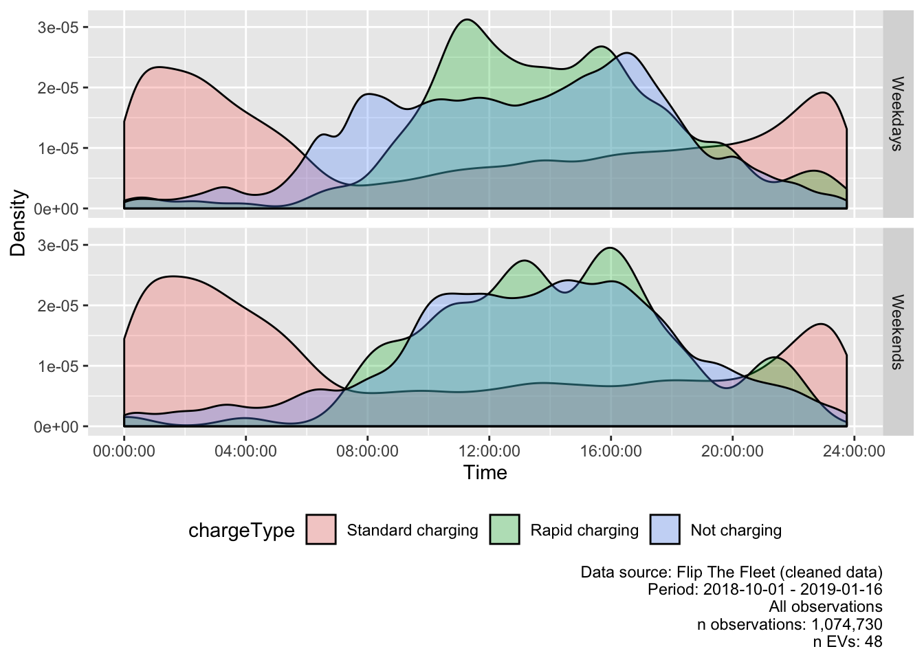
Figure 5.3: Density plot of charging start times during weekdays

In general, these results indicate that the greatest frequency of standard charging events occurs between 20:00 and 08:00, with very low occurrences of charging during morning and evening grid peaks. Rapid charging on the other hand is a day-time activity on both weekdays and weekends.

To make the patterns of ‘initial charging’ clearer, we use just the ‘first’ charge observation in a pair (see above) and also exclude automatic battery ‘top-ups’ (refer to Section 5.3) by filtering out any data where a charging observation begins while the state of charge is greater than 90%. Having done so, Figure 5.4 shows the distribution of the start of ‘charge sequences’ and shows that the number of charging event starts increases steadily through the day before an apparent brief lull between 19:00 and 21:00 and then increases substantially thereafter.

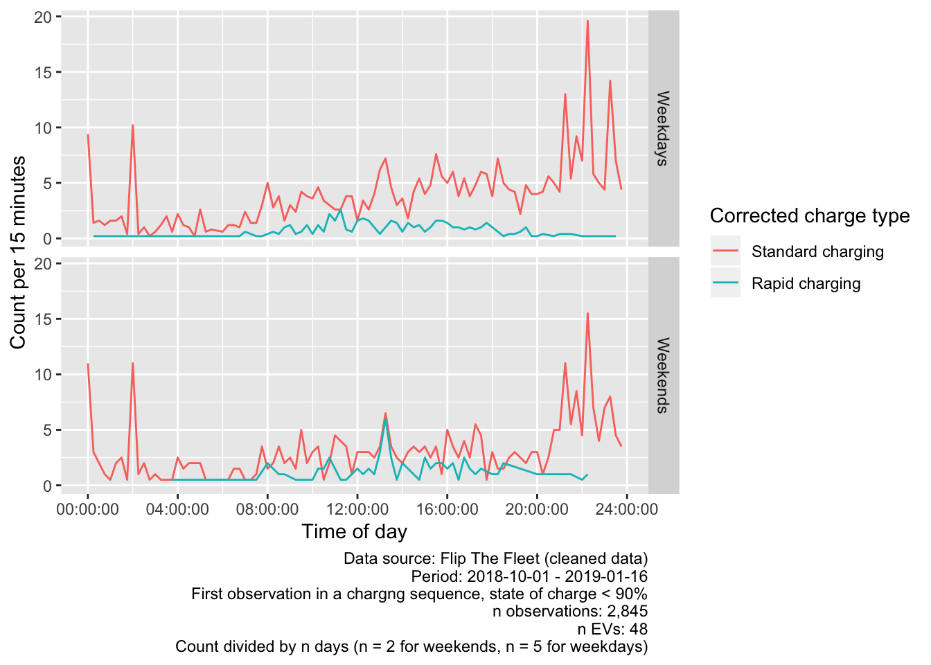
Figure 5.4: Charging start times where state of charge < 90%

Figure 5.5 uses a density plot to represent the proportion of charging sequences that start at different times of the day on weekdays vs weekends for standard and rapid charging (corrected classification).

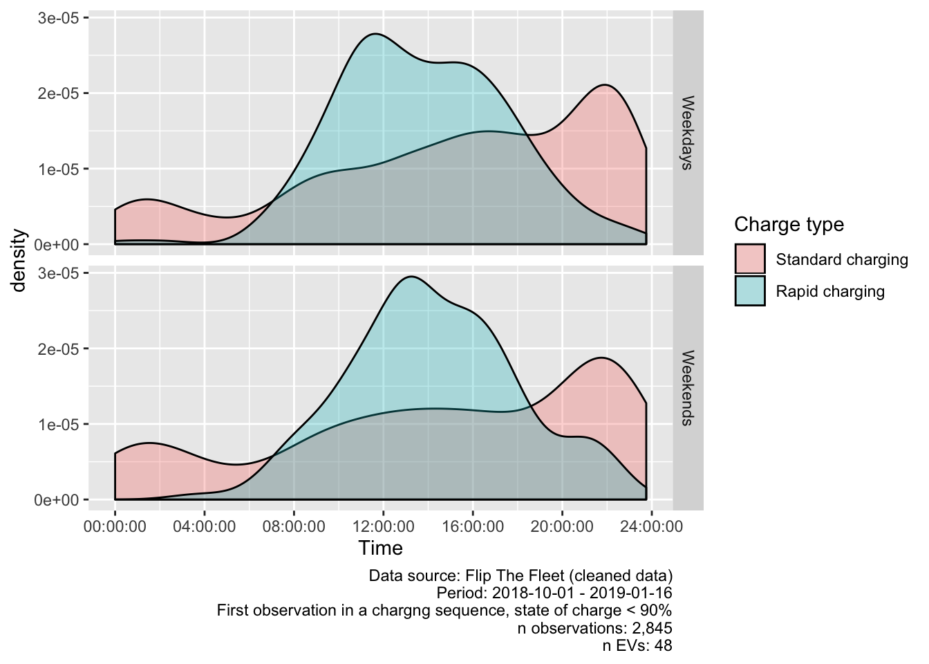
Figure 5.5: Density plot of charging start times where state of charge < 90%

As we can see, standard charging sequences (as opposed to single observations) have a noticeably different profile to charging patterns for rapid charges. It suggests that the largest number of standard charging events start between 20:00 and 22:00 and run overnight, and perhaps use the more powerful public charge points to top up during the day. However the plot also show a substantial proportion of charging events start earlier in the day, including during the NZ peak demand periods of 07:00 - 09:00 and 17:00 - 21:00.

Standard charging events were most likely to begin around 10pm during both weekdays and weekends. As it seems unlikely that this is due to vehicle drivers returning home at this hour, this effect may be due to drivers setting the charger on a timer to take advantage of cheaper “off-peak” electricity times, which frequently begin around 10pm.

Rapid charging events were most likely to begin at 11:30am on weekdays and 1pm during weekends.

The lack of data from EVs which are neither charging nor being driven means that it is impossible to directly calculate the proportion of the sample who were charging at a given time. Instead we can estimate the proportion of EVs which were charging by:

• counting the number of EVs (nEVs) that were observed to charge for each charge type in each quarter hour of every day;
• counting the total number of EVs (totalDayEVS) that were recorded charging or not charging (i.e. in use) on that day. Since we would receive no data from EVs that were not in use and not charged on a given day, this is the best estimate we can make of the EV ‘live population’ on a given day;
• calculating the % charging for each charge type for each quarter hour of every day = nEVs/totalDayEVS;
• calculating the mean of this value across all weekdays and weekend days for each charge type.

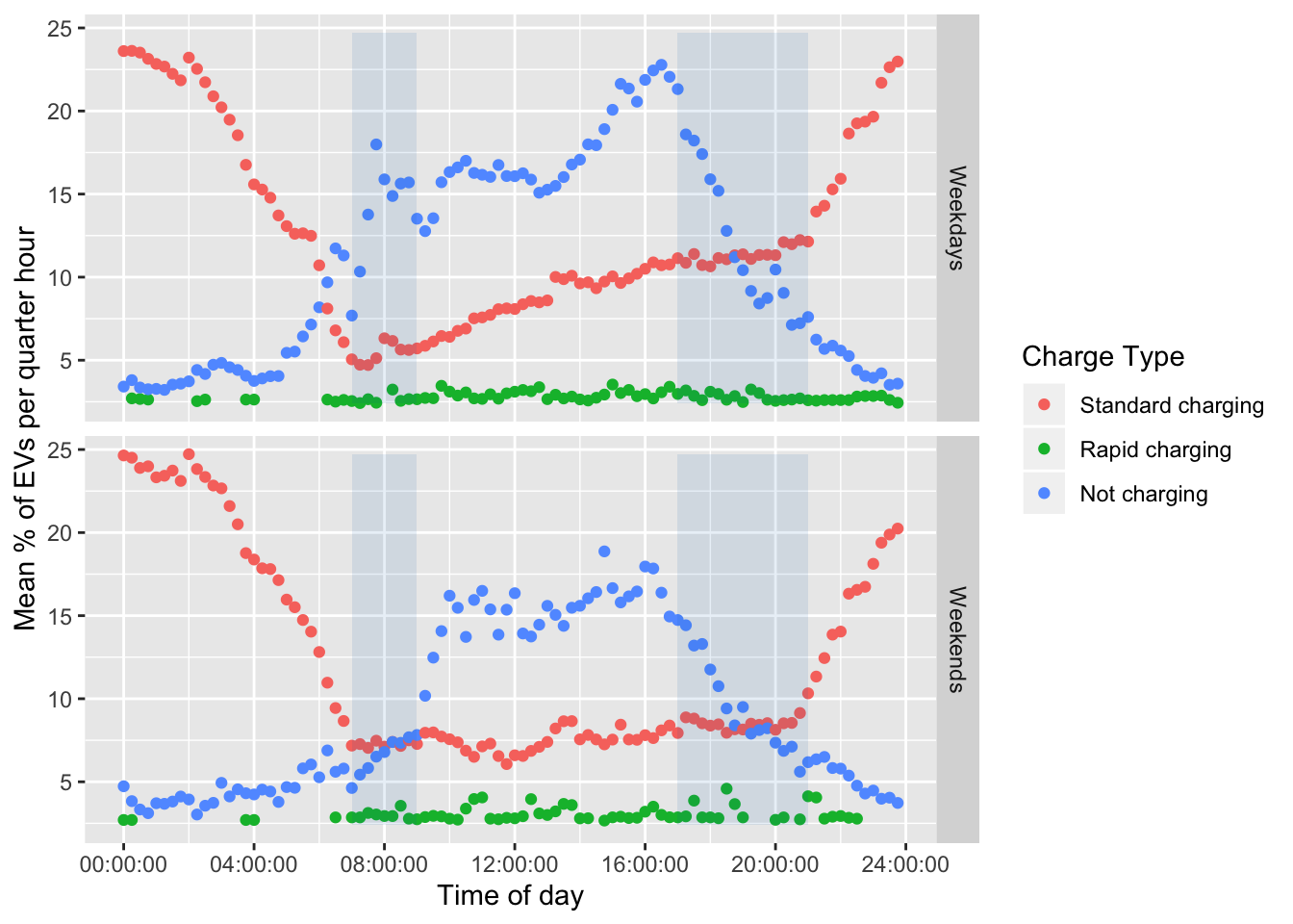
Figure 5.6: Percent of vehicles charging in a given 15 minute period

These results are reported in Figure 5.6 which shows the estimated mean % of EVs which were charging in each quarter-hour of the day by charge type. As we would expect the pattern of charging replicates that found in Figure 5.1 and indicates the relative rarity of rapid charging.

5.2 Charging duration

This section analyses the duration of observed charging events to understand when longer charging sequences are likely to occur. Table 5.1 shows the mean durations for all all charging events by event start time for standard charging durations greater than 8 minutes (see Section 4.3.2) and all rapid charging events.

Table 5.1: Mean duration of charge events by charge type (filtered data, corrected charge type)

chargeTypeCorrected	mean	median	min	max	sd
Standard charging	243.01 mins	207.12 mins	8.03 mins	1616.72 mins	190.61
Rapid charging	20.69 mins	14.26 mins	0.02 mins	582.53 mins	42.39

Table 5.2: Mean duration of charge sequences (values > 480 minutes)

qHour	chargeTypeCorrected	weekdays	meanDuration	nEVs
10:30:00	Standard charging	Weekends	1324.10 mins	1
02:30:00	Standard charging	Weekends	528.46 mins	4

Figure 5.7 plots the mean duration by time of day and weekday vs weekend and charge type. As before we use transparency to indicate the number of unique EVs contributing to the mean values and we have removed a small number of very large duration outliers (mean duration > 540 minutes or 9 hours) which appears to be based on just 1 or 2 EVs (see Table @ref:(tab:makeDurationTimeMean)).

As we would expect, the plot shows that for standard charging mean ‘forward’ duration generally decreases from midnight, presumably as batteries are becoming fully charged through to 06:00 and then increases as the time of starting to charge increases through the day before trending downwards before midnight. Again, this confirms that charge events starting in or just after the evening peak demand period on both weekdays and weekends are likely to be longer, possibly reflecting the lower state of charge at this time of day (following use).

Duration of rapid charge events by start time appear to be more randomly distributed, although very few events were recorded between midnight and 7am. This, along with the comparatively low number of recorded rapid charge events indicated in Fig. 4.4 suggests that drivers utilize rapid charging only “as necessary” to ensure they have enough battery capacity to complete their journey or when ‘at work’ or conducting some other mobility related task such as shopping.

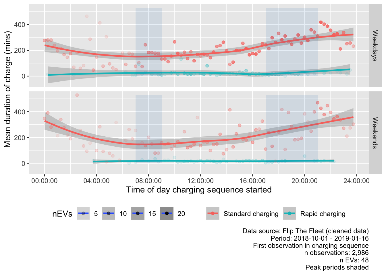
Figure 5.7: Mean duration (within quarter hours) by time of charging start

5.3 State of charge

The state of charge is the percentage of energy still available to be used in the battery. In future, electric vehicles may be able to discharge any remaining battery charge as electricity into the grid, a process known as vehicle to grid (V2G) energy transfer. This may allow electric vehicles to have a net beneficial effect on the grid, reducing the evening peaks by providing electricity to the home during this period, and then recharging later in the evening or early the next morning when peak demand has diminished.

5.3.1 Start of charging sequence

This section provides an indication of the state of charge of electric vehicles when they start charging, so that the potential of V2G technology can be assessed.

Table 5.3: Summary statistics for % state of charge on first charge in a sequence

Charge Type	Period	Mean SoC %	Median SoC %	n Obs	n EVs
Standard charging	Early morning	89.89	97.75	2500	41
Standard charging	Morning peak	80.43	97.00	425	39
Standard charging	Day time	69.01	67.03	1536	47
Standard charging	Evening peak	70.37	75.67	946	43
Standard charging	Late evening	64.35	57.32	1112	38
Rapid charging	Early morning	39.09	39.88	6	5
Rapid charging	Morning peak	45.42	42.86	27	9
Rapid charging	Day time	44.32	43.30	263	37
Rapid charging	Evening peak	43.69	39.25	67	25
Rapid charging	Late evening	39.30	39.14	18	9

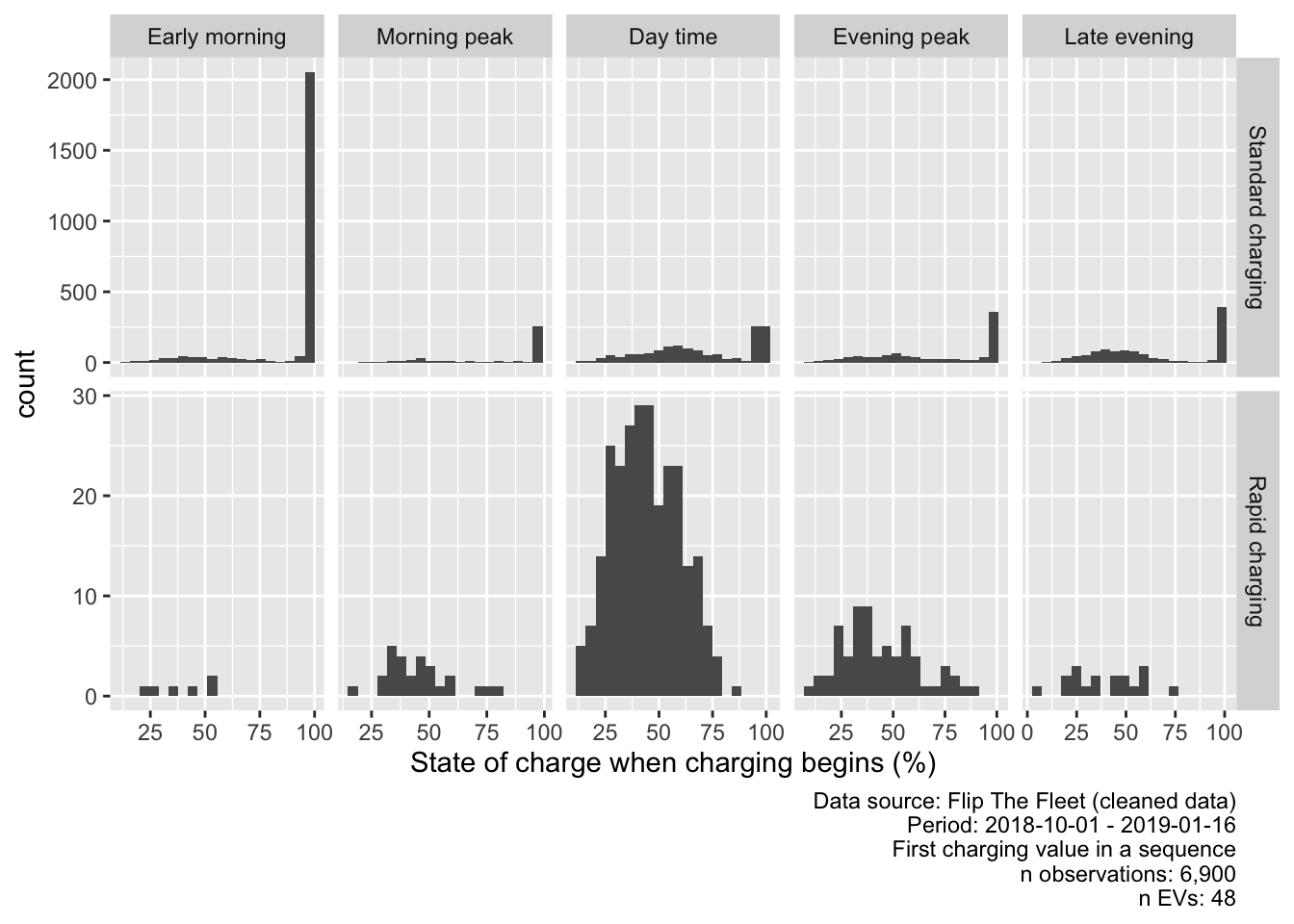
Figure 5.8: Value of state of charge (first charging observation)

As can be seen in Figure 5.8, using the cleaned complete observations data, the state of charge for the majority of standard charge observations is above 90%. This is most likely due to the manner in which the charger regularly turns off and on again near the end of the charging cycle as described in Section 4.2.

Figure 5.9 shows the state of charge values for all charging events but with state of charge greater than 90% removed from the data for clarity. The figure indicates that many vehicles begin charging despite having greater than 50% charge remaining. This has clear implications for battery life management since continually top-up charging is known to substantially shorten the lifetime of EV batteries (XX ref needed XX). However it also indicates the potential to use the charge in the battery to feed into the grid, especially in the residential context.

Table 5.4: Summary statistics for % state of charge on first charge in a sequence, values > 90% removed

Charge Type	Period	Mean SoC %	Median SoC %	n Obs	n EVs
Standard charging	Early morning	49.45	47.68	398	33
Standard charging	Morning peak	52.70	48.95	161	31
Standard charging	Day time	54.39	55.42	1013	47
Standard charging	Evening peak	50.48	50.56	543	43
Standard charging	Late evening	44.93	44.36	700	36
Rapid charging	Early morning	39.09	39.88	6	5
Rapid charging	Morning peak	45.42	42.86	27	9
Rapid charging	Day time	44.32	43.30	263	37
Rapid charging	Evening peak	43.69	39.25	67	25
Rapid charging	Late evening	39.30	39.14	18	9

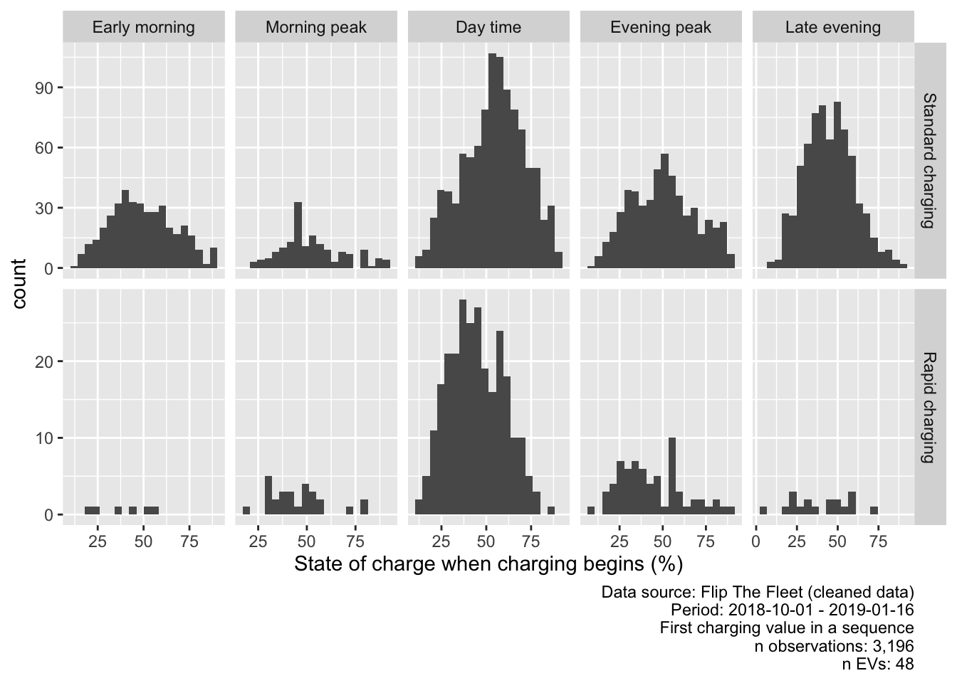
Figure 5.9: Value of state of charge when charging begins (values > 90% removed)

Figure 5.10 repeats this analysis but uses the cleaned and corrected inferred start/end of charging sequence data instead of all charging observations. Figure ?? shows very similar distributions to the previous ‘all-observations’ plot (Figure 5.8) and confirms that sequences of standard charging in particular most frequently start with battery state of charge over 50%.

Table 5.5: Summary statistics for % state of charge on first charge in a sequence, chargeType corrected, values > 90% removed

Charge Type	Period	Mean SoC %	Median SoC %	n Obs	n EVs
Standard charging	Early morning	45.86	45.06	344	31
Standard charging	Morning peak	51.62	47.27	136	28
Standard charging	Day time	52.44	53.87	861	47
Standard charging	Evening peak	48.63	48.88	461	40
Standard charging	Late evening	44.47	43.63	664	36
Rapid charging	Early morning	39.09	39.88	6	5
Rapid charging	Morning peak	45.42	42.86	27	9
Rapid charging	Day time	44.16	43.25	261	36
Rapid charging	Evening peak	43.69	39.25	67	25
Rapid charging	Late evening	39.30	39.14	18	9

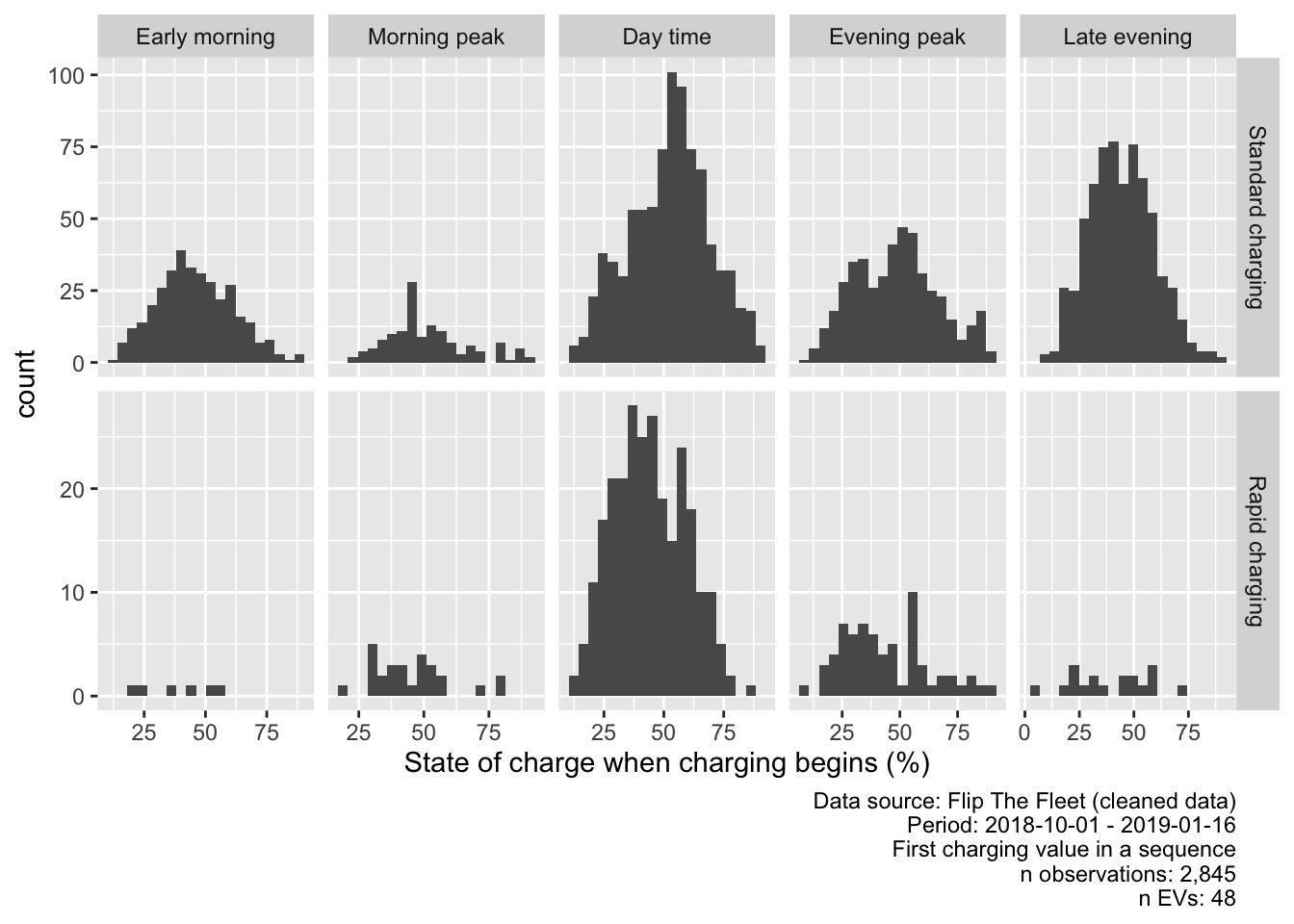
Figure 5.10: Value of state of charge at beginning of charging sequence (chargeType corrected, values > 90% removed)

Statistics:

• 1 of the 379 rapid charging sequences with intial SoC < 90% started with less than 5% charge;
• 132 of 379 (34.83%) rapid charging sequences with intial SoC < 90% started with greater than 50% charge;
• 1166 of 2466 (47.28%) standard charging sequences with intial SoC < 90% started with greater than 50% charge;

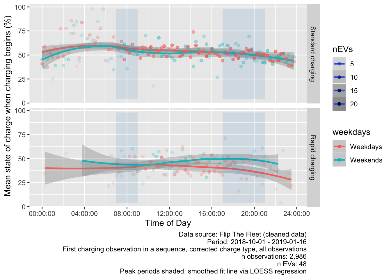
Figure 5.11: Mean state of charge at beginning of charge sequence by time of day (chargeType corrected, all observations)

Finally, Figure 5.11 shows the mean % charge at the time of first charging observation in a sequence using the cleaned and corrected inferred start/end of charging sequence data. This includes all events, even the brief ‘top-up’ early morning events to indicate when the stored energy is available at the start of a charge sequence.

The plot suggests that available capacity may be relatively stable throughout the day albiet with a higher mean capacity around the morning peak as we would expect given over-night charging. It is unlikely that this early morning capacity would be willingly made available for V2G since the EV may be used in the near future although this may not always be the case. However it is interesting to note that mean capacity at start of charge in the evening peak period is still roughly 50% indicating relatively good power availability even when we might expect the vehicle to have recently returned home.

Making the assumption that each EV has a 24 kWh battery we can calculate the available kWh at the start of each charge for V2G purposes. This is shown in Table 5.6 and Figure 5.12.

Table 5.6: Estimated kWh available by time period and charge type

chargeType	peakPeriod	meankWh	sdkWh	nObs	nEVS
Standard charging	Early morning	11.01	3.68	344	31
Standard charging	Morning peak	12.39	3.80	136	28
Standard charging	Day time	12.58	4.02	861	47
Standard charging	Evening peak	11.67	4.36	461	40
Standard charging	Late evening	10.67	3.57	664	36
Rapid charging	Early morning	9.38	3.47	6	5
Rapid charging	Morning peak	10.90	3.55	27	9
Rapid charging	Day time	10.60	3.64	261	36
Rapid charging	Evening peak	10.49	4.45	67	25
Rapid charging	Late evening	9.43	4.34	18	9

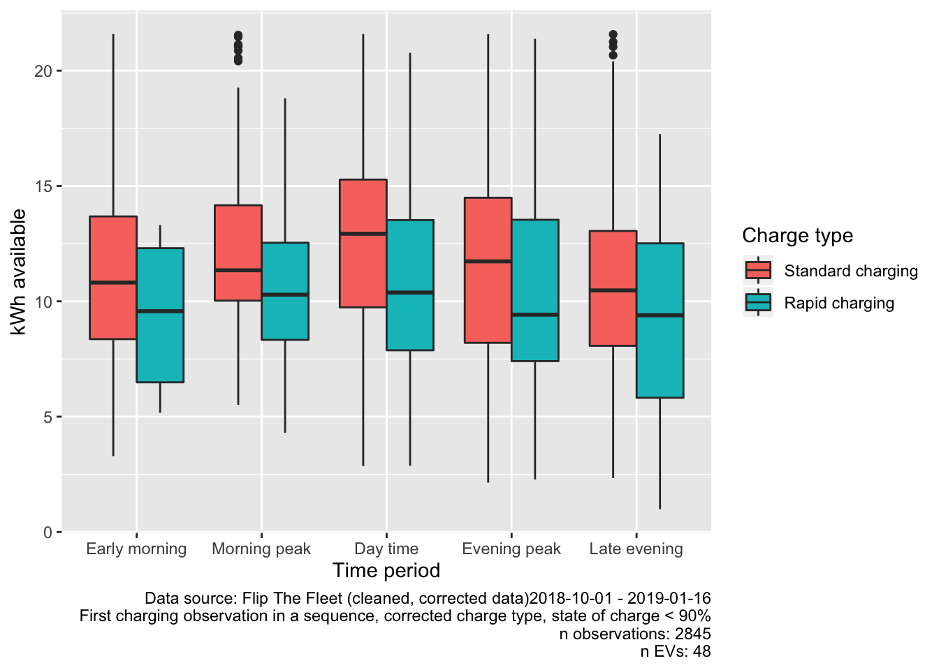
Figure 5.12: Estimates of available kWh by time period

These show, for example, that the mean kWh available during the evening peak period is 11.67 with a range of 2.14 to 21.58 kWh. We can also see that similar values are available in the morning peak period but further analysis would be required to estimate how much of this could be used during the period without impacting subsequent use. Other analyses could include:

• estimating the overall kWh available at any given time for co-ordinated demand response purposes;
• estimating the effect of different demand response or V2G uses of the battery capacity on the patterns of use before next charge assuming no change in usage behaviour to that observed;
• estimating similar effects under scenarios of behavioural change (charging in response etc)

Of course if we knew exactly what the battery capacity was for each vehicle we could calculate a far more accurate estimate.

5.3.2 End of charging sequence

Figure 5.13 shows the state of charge at the end of a charging sequence using the cleaned and corrected inferred start/end of charging sequence data, We can now see that the majority of standard charge sequences end with close to 100% charge but most rapid charge sequences end with around 75-80% charge.

Table 5.7: Summary statistics for % state of charge on last charge in a sequence

Charge Type (corrected)	Mean SoC %	Median SoC %	n Obs	n EVs
Standard charging	90.71	97.30	6575	47
Rapid charging	72.39	75.02	323	39

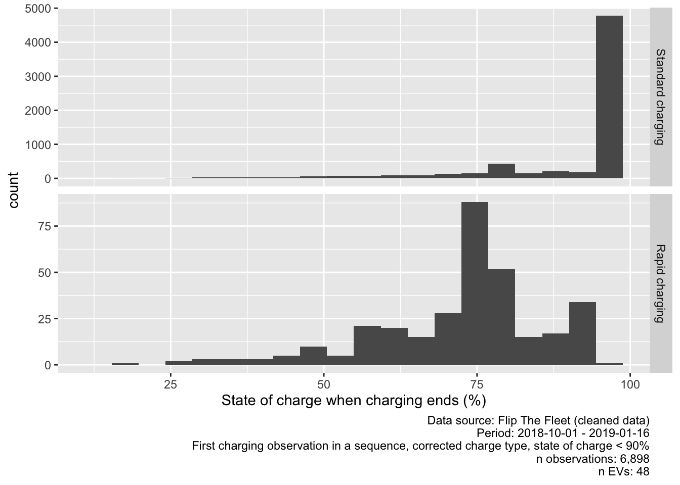
Figure 5.13: Value of state of charge at end of charging sequence (chargeType corrected, all values

Figure 5.14 shows the difference in charge gain for all charge sequences where the starting charge was less than 90% (as above).

Table 5.8: Summary statistics for % state of charge gain by last charge in a sequence

Charge Type (corrected)	Mean SoC gain %	Median SoC gain %	n Obs	n EVs
Standard charging	31.46	32.77	2801	47
Rapid charging	30.30	29.67	395	41

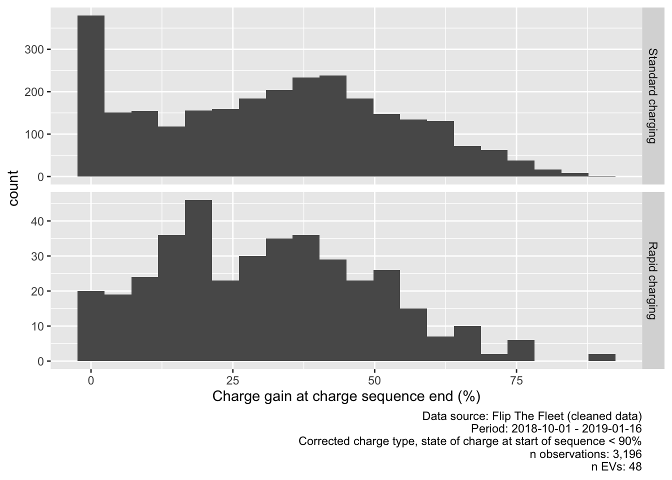
Figure 5.14: Charge gain during charging sequence (chargeType corrected, all values

5.4 Patterns of power demand

Given this distribution of charging events, it is important to understand their magnitude to understand the potential effect on the electricity network. Although we are hampered by the lack of observations when the EV is inactive, this section analyses the patterns of power demand for the observations we have.

Overall 75% of standard charging observations were 1.46 kW or more but the figure was 19.88 kW or more for rapid charging.

The remaining results in this section are experimental and preliminary. Use with care (if at all) or just skip to the next section (5.5).

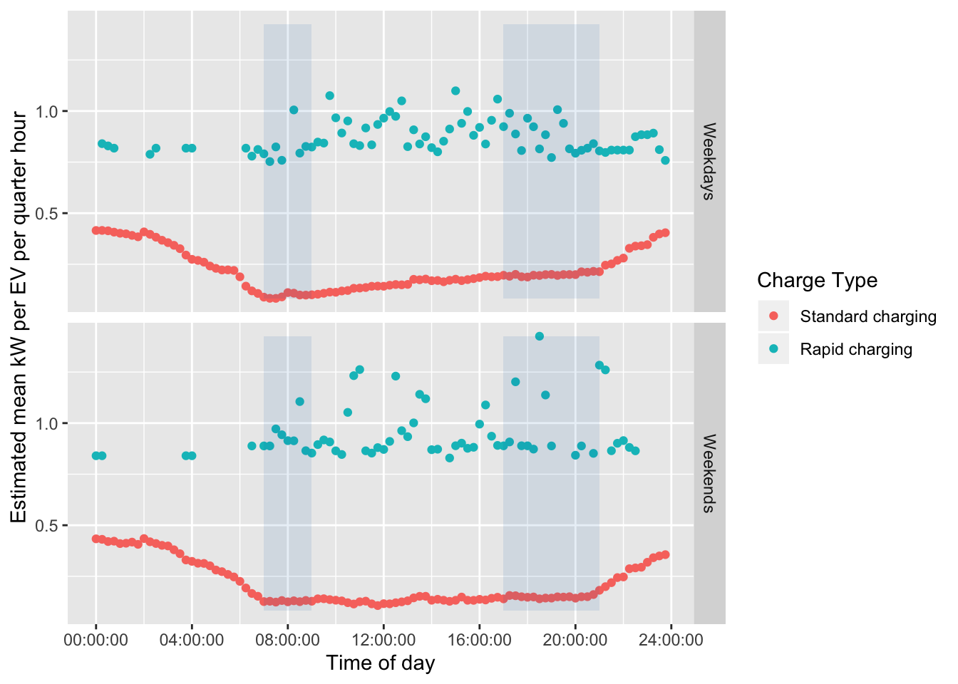
Figure 5.15 shows the mean charging demand in kW calculated across all observations after setting rapid charge observations to 0 kW. As we would expect the kW load due to the EVs follows essentially the same shape as the charging event proportions shown above but with slightly more evidence of a 13:00 and 16:00 mini-peak and distinct differences between weekday and weekend mornings. As before, the apparent rapid increase in demand (and the pre-20:00 spike) are more likely to be due to decreasing numbers of ‘non-charging’ observations than increases in charging (see Figure 5.3.

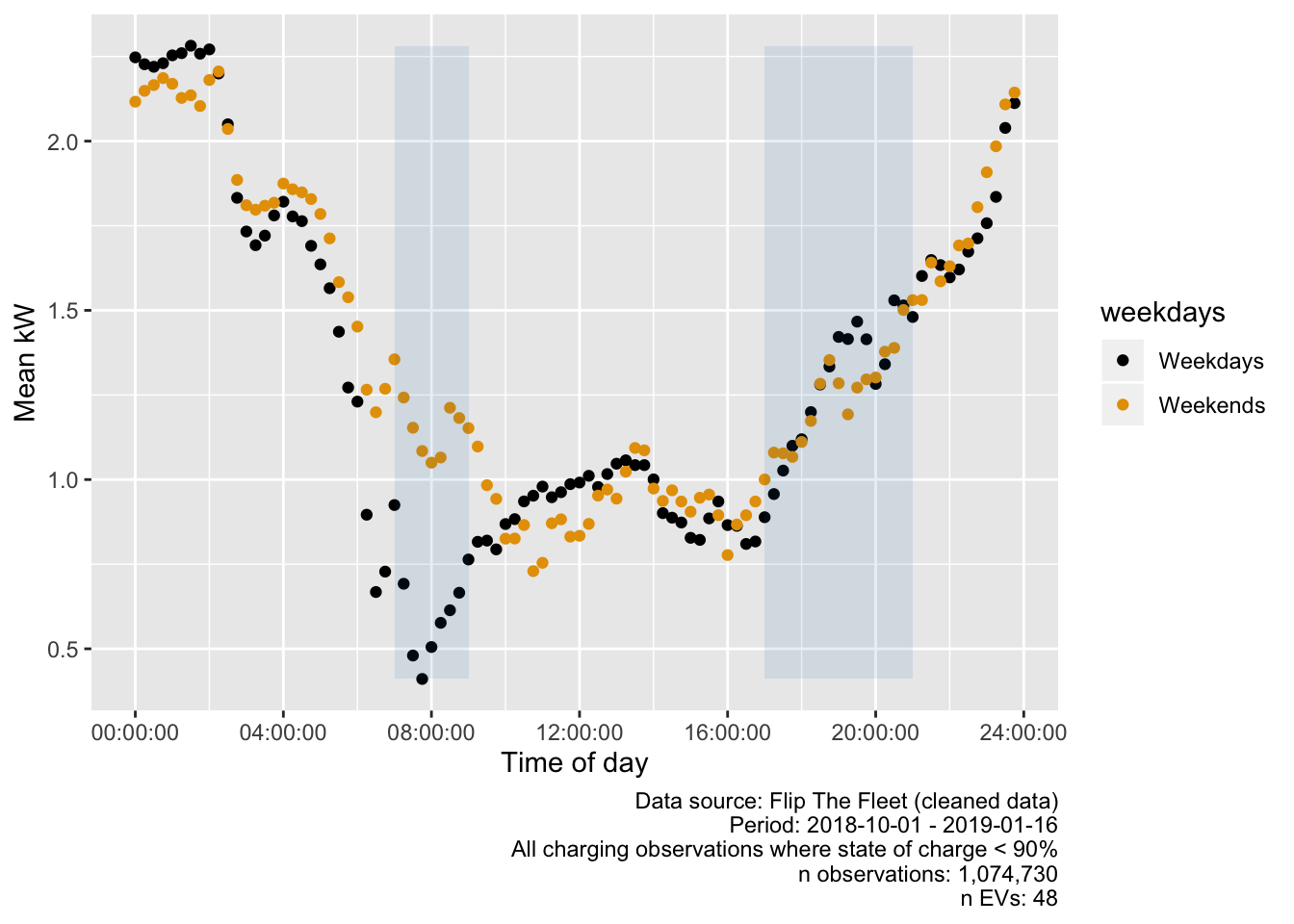
Figure 5.15: Mean kW per quarter hour (treating rapid charging as 0 kW)

Figure 5.16 repeats Figure 5.15 but shows the mean charging demand in kW calculated across all observations after setting standard charge observations to 0 kW. Again, the kW load due to the EVs follows essentially the same shape as the charging event counts shown above and the low mean value should remind us that rapid charging was relatively rare in the data.

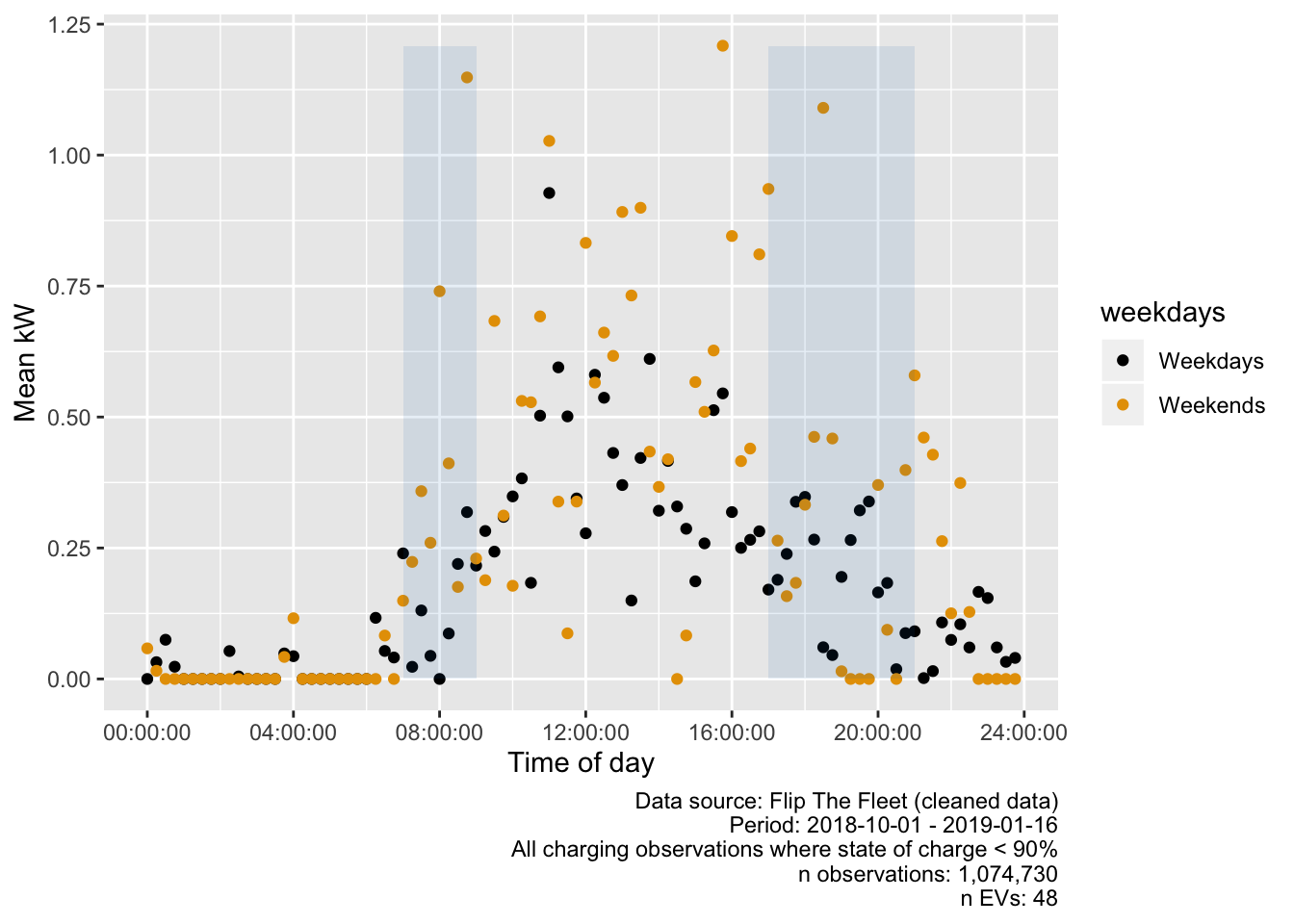
Figure 5.16: Mean kW per quarter hour (treating standard charging as 0 kW)

In next plots we use transparency to indicate the number of EVs contributing to each of the mean calculations to give a guide to their reliability and indicate the relative proportion of sample EVs that contribute to each mean value. Dots with stronger colours indicate means calculated from a larger number of EVs and, given the data gaps noted in Section 4.1, this therefore indicates patterns which are generally shared across a larger number of EVs. We would therefore expect darker dots (most vehicles) durng overnight charge times and lighter plots (fewer vehicles co-incidentally charging) through the day.

Figure 5.17 shows the mean power demand for standard charging observations by time of day and weekdays vs weekends for the selected time period. This plot appears to show that there are three peaks in standard charging, one at 10:00, one at 18:00 (possibly based on fewer EVs) and one after midnight on weekdays. There are also noticeable 07:00 and 16:00 charging blips. On the other hand at weekends the daytime peak shifts to 14:00. Thus, while our previous analysis suggested that charging events were more likely to start later in the evening, the power demand of earlier charging events may actually be relatively high and co-incide with existing peak demand periods.

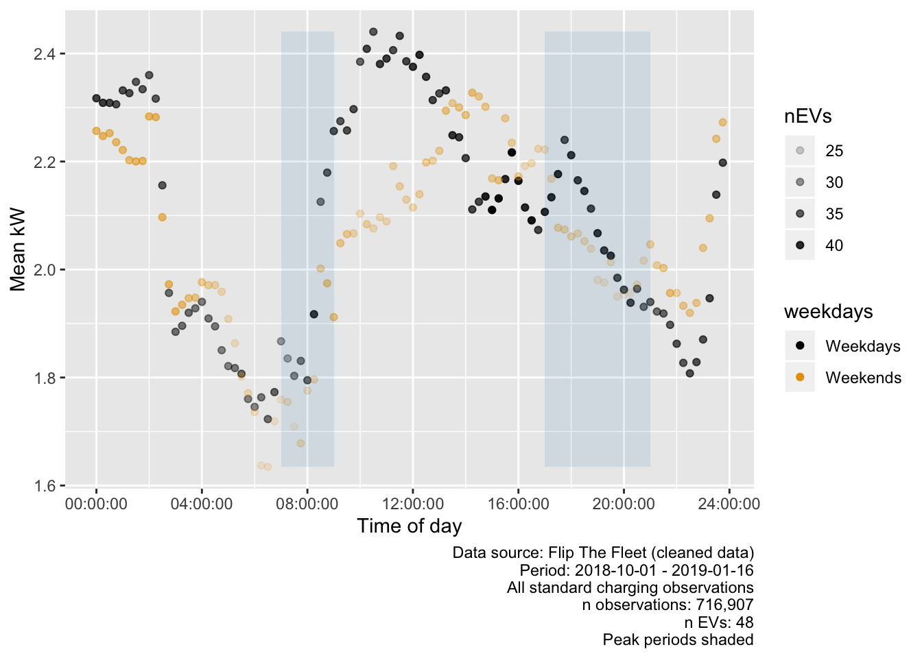
Figure 5.17: Mean charging power demand (kW) by time of day (‘standard’ charging)

Rapid charging however has no detectable pattern other than a clear increase in density during weekday daytimes (Figure 5.18). However, we can now see the effect that rapid charging may have with significant EV uptake.

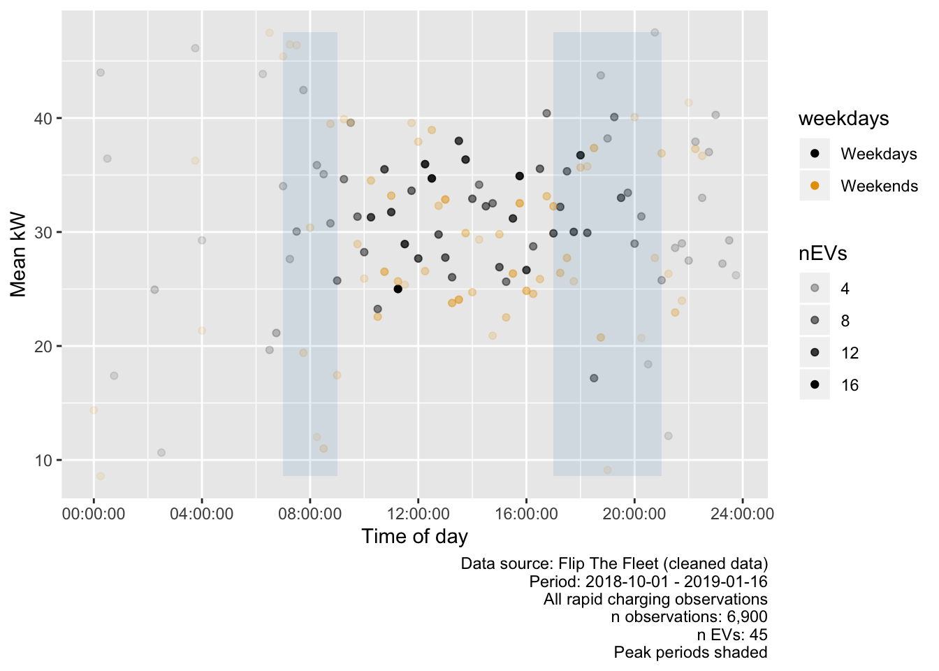
Figure 5.18: Mean charging power demand (kW) by time of day (‘rapid’ charging)

It is possible that the ‘standard charge’ day-time peak is skewed by mis-classified short low power ‘Rapid charge’ observations (see Section 4.3.1). Figure 5.19 attempts to allow for this misclassification by plotting the median rather than the mean. The plot more clearly shows the 10:00 weekday spike which, if we assume that the mis-classified ‘Rapid charges’ will be skewing the standard charge mean value upwards, is likely to be due to mis-classified ‘Rapid charging’. However the 18:00 peak persists as does the 14:00 weekend peak while overnight charging levels are relatively stable as we would expect from 5.17.

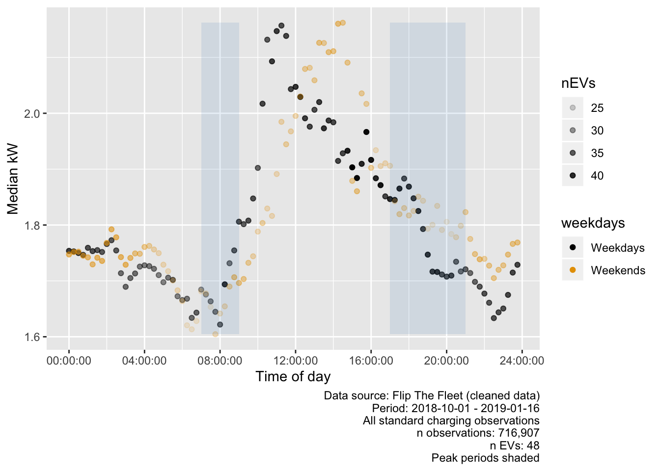
Figure 5.19: Median charging power demand (kW) by time of day

Figure 5.20 repeats the median power-based analysis for ‘Standard charging’ but shows the results by month. While the sample size is probably too small to draw robust conclusions there appear to be differences between months with December showing few discernable peaks and September and January showing much lower daytime weekday charging. In addition, weekdays and weekends are much more similar in November and December.

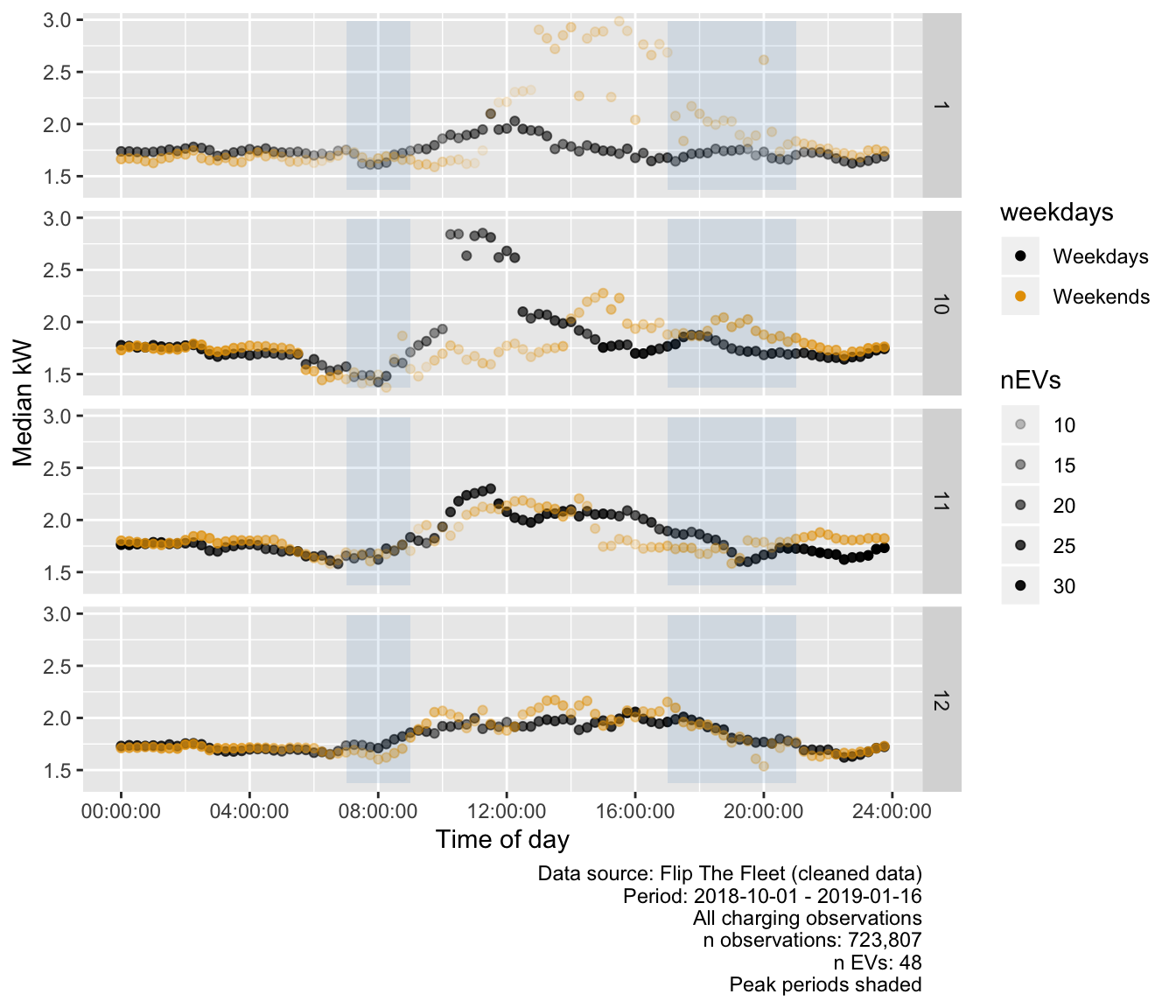
Figure 5.20: Median charging power demand (kW) by time of day and month

5.4.1 Power demand summary

On face value the results suggest that EVs could be placing additional power demand on local and national networks during well-known periods of peak demand although this appears to vary by month for this small sample of EV owners.

Clearly this analysis should be revisited once the potential misclassification of ‘rapid’ as ‘standard’ charging observations has been resolved and the ‘missing’ non-use (zero charging) observations have been imputed.

5.5 Imputing power demand

The lack of data from EVs which are neither charging nor being driven means that it is difficult to directly estimate the ‘average’ power demand for the sample. Instead we use two different approaches:

• an estimate of the proportion of EVs which were charging and our derived median ‘standard’ and ‘rapid’ kW demand to estimate these values;
• an estimate based on aggregating demand to half-hours.

5.5.1 Method 1: Imptation based on sample charging proportions

Warning: we think this method is incorrect. Do not use results in this section. Jump to Section 5.5.2

Based on Table 4.5, let us assume:

• standard charging = 1.76 kW (median)
• rapid charging = 31.09 kW (median)

We can now calculate the mean kW demand per EV per time period by multiplying these values by the appropriate % of EVs who were charging by charge type (the data used to construct 5.6). The results of doing so are shown in ??.

We can now see that:

• standard charging places a relatively low additional mean kW load on the electricity network which is generall highest outside peak demand periods. However there is some evidence of an upward trend from ~ 16:00 through to 21:00.
• despite the relative rarity of rapid charging, their much higher power demand produces a much higher mean kW load on the network, especially during the day. Note that the level of rapid charging between 00:00 and 08:00 on weekdays seems unexpected although it is reflected in Figure 5.6 which shows that it is based on 7 different EVs. Given the relatively low number of EVs reporting rapooid charging in this time period, this result should be treated with caution.

5.5.2 Method 2: Half-hourly aggregation

In this method we:

• set the dateTime of each observation to exactly 1 minute by setting dateTime_1min = floor(dateTime) - so e.g. 2018-10-01 20:00:59 -> 2018-10-01 20:00. This may create multiple observations per EV where more than 1 observation was taken within a given minute;
• calculate the mean kW per date-hour-minute per chargeType for all dateTime_1min times per EV. In most cases this is a mean of a single value but in those cases where there is more than 1 observation per minute it will be a mean of those observations;

Table 5.9: Summary of floor(1 minute) aggregate data

	dvID	r_dateTime1MinFl	chargeType	peakPeriod	weekdays	meankW	nObs
	Length:897040	Min. :2018-10-01 13:00:00	Standard charging:599082	Early morning:297815	Length:897040	Min. : 0.000	Min. :1.000
	Class :character	1st Qu.:2018-10-28 22:57:00	Rapid charging : 5793	Morning peak : 49789	Class :character	1st Qu.: 0.000	1st Qu.:1.000
	Mode :character	Median :2018-11-22 15:30:00	Not charging :292165	Day time :290047	Mode :character	Median : 1.475	Median :1.000
	NA	Mean :2018-11-22 21:10:05	NA	Evening peak :136428	NA	Mean : 1.592	Mean :1.198
	NA	3rd Qu.:2018-12-17 12:05:00	NA	Late evening :122961	NA	3rd Qu.: 1.924	3rd Qu.:1.000
	NA	Max. :2019-01-16 12:59:00	NA	NA	NA	Max. :70.164	Max. :6.000

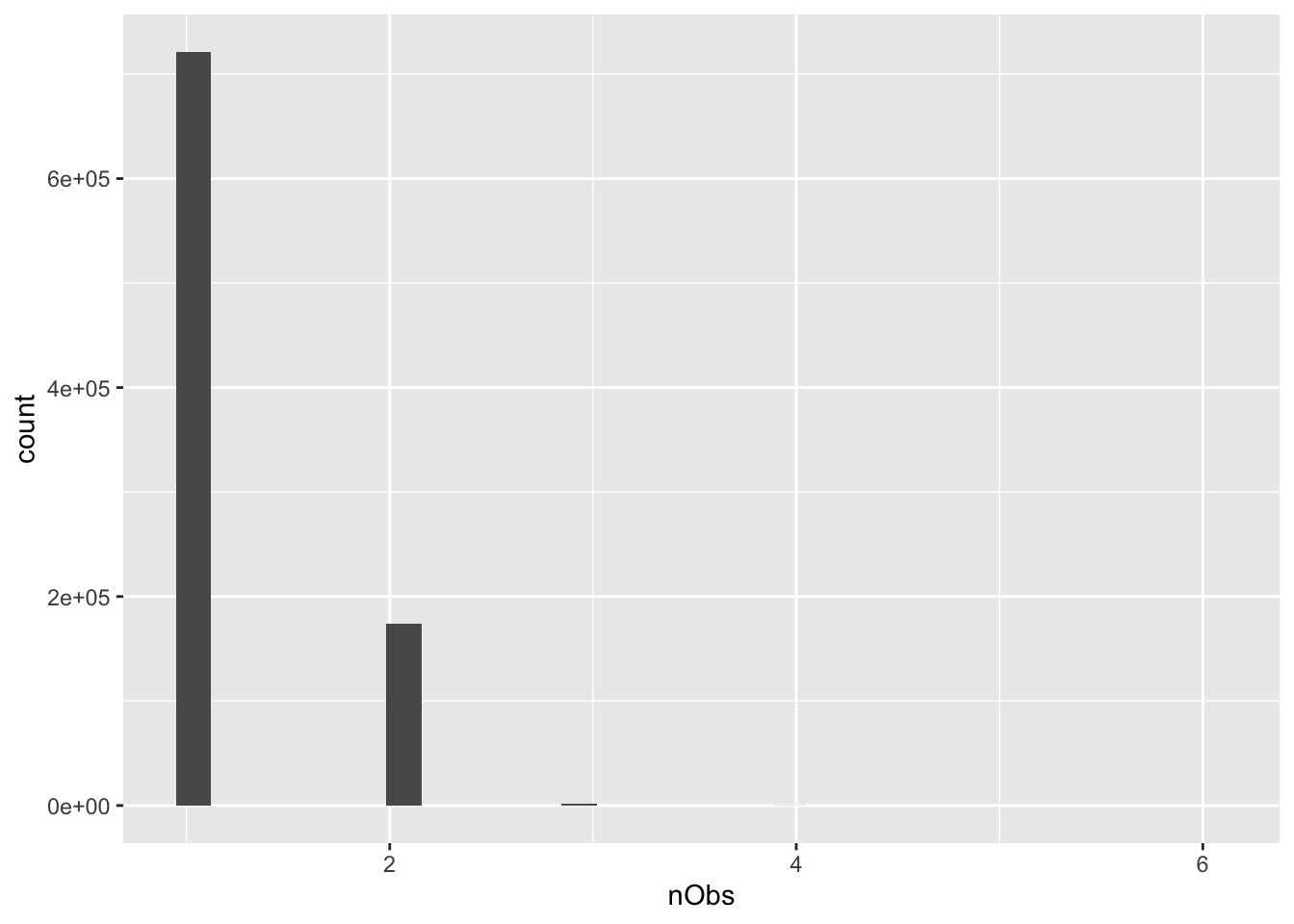
Figure 5.21: Histogram of number of observations per aggregated floor(1 minute) date time per EV

Next we:

• sum the mean kW per date-half-hour by chargeType and divide by 30 to give mean kW for the half-hour

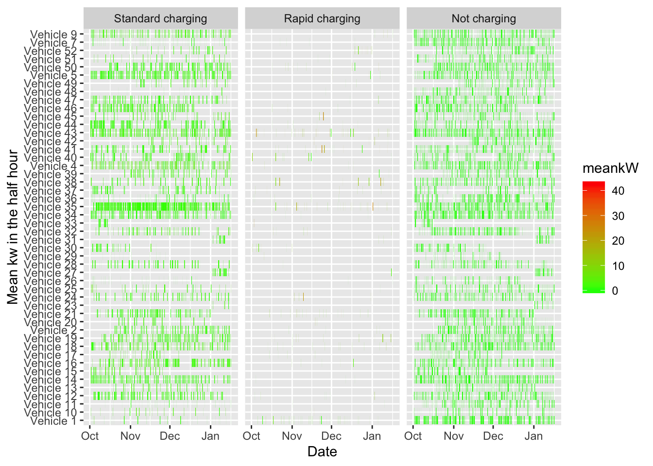
Figure 5.22: Half-hourly mean kW for all EVs - testing for missing data

NB: calculating a mean across these half-hourly observations requires knowing how many half-hours are missing and so can be set to 0.

tbc

5.6 Estimating energy consumption

In addition to electricity demand (power in kW) we are also interested in overall energy consumption (kWh). To do this we use two methods based on the two approaches to estimating kW above.

5.6.1 Method 1: proportions charging

Warning: we think this method is incorrect. Do not use results in this section. Jump to Section 5.6.2

In the first method, we take the mean kW per quarter hour per EV values reported in ?? and divide them by 4 to give mean kWh per quarter hour per EV.

Table 5.10: Estimated mean daily kWh by charge type (all observations)

Day	Charge type	Total mean kWh	% total mean kWh (within day)
Weekdays	Standard charging	5.30	24.02
Weekdays	Rapid charging	16.77	75.98
Weekends	Standard charging	5.12	25.44
Weekends	Rapid charging	15.01	74.56

Overall we estimate that 24.69% of electricty consumption for EVs is via standard charging. Table 5.10 reports the estimated mean daily kWh consumed during charging on weekdays and weekends and the % within weekdays and weekends. The results indicate little difference between weekdays and weekends in terms of the % of kWh consumption which is standard vs rapid charging.

Table 5.11: Estimate mean kW and kWh by charge type and peak period (all observations)

Day	Peak period	Charge type	Total mean kWh	% total mean kWh (within day)
Weekdays	Early morning	Standard charging	2.15	9.74
Weekdays	Early morning	Rapid charging	2.03	9.22
Weekdays	Morning peak	Standard charging	0.19	0.86
Weekdays	Morning peak	Rapid charging	1.44	6.52
Weekdays	Day time	Standard charging	1.22	5.51
Weekdays	Day time	Rapid charging	7.32	33.15
Weekdays	Evening peak	Standard charging	0.80	3.61
Weekdays	Evening peak	Rapid charging	3.50	15.84
Weekdays	Late evening	Standard charging	0.95	4.30
Weekdays	Late evening	Rapid charging	2.49	11.26
Weekends	Early morning	Standard charging	2.38	11.85
Weekends	Early morning	Rapid charging	1.06	5.28
Weekends	Morning peak	Standard charging	0.26	1.27
Weekends	Morning peak	Rapid charging	1.87	9.30
Weekends	Day time	Standard charging	1.05	5.23
Weekends	Day time	Rapid charging	7.41	36.81
Weekends	Evening peak	Standard charging	0.59	2.95
Weekends	Evening peak	Rapid charging	2.92	14.51
Weekends	Late evening	Standard charging	0.83	4.14
Weekends	Late evening	Rapid charging	1.74	8.66

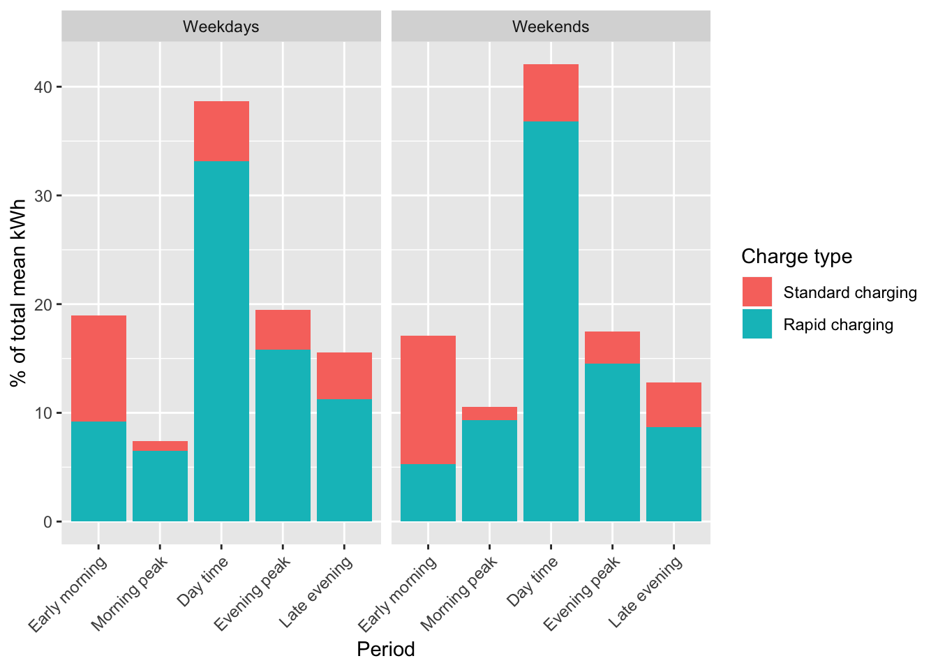
Figure 5.23: % total mean kWh consumption per EV

Table 5.11 and Figure 5.11 repeats this analysis but shows the results by peak period. Clearly rapid charging during the day dominates energy (kWh) consumption with standard charging during the evening peak being responsible for a mere 3-4% of the energy consumed by EV charging.

5.6.2 Method 2: Aggregation

Here we take the floor(1 min) data described in Section 5.5.2 and:

• divide this by 2 to give the mean kWh per date-half-hour

Next we simply sum these kWh values across all observations for different categories to get some idea of the relative proportions of energy being drawn in different contexts and charging situations

Figure 5.24 shows the results of doing this for weekends and weekdays. Note that the totals have been ‘normalised’ to allow for the different numbers of weekdays vs weekend days but we make no checks as to whether the ‘right’ number of weekdays and weekend days are represented in the data (e.g. where we received no data due to inactivity - see above). This shows that the patterns of weekday vs weekend energy consumption are similar with overnight standard charging dominating. Consumption during morning peak periods is low but slightly higher in the evening peaks as the charging timing results above would imply. Rapid charging plays a larger role in day-time energy consumption but it’s rarity means that despite higher power demand (kW) it’s energy impact (kWh) is relatively low in this sample.

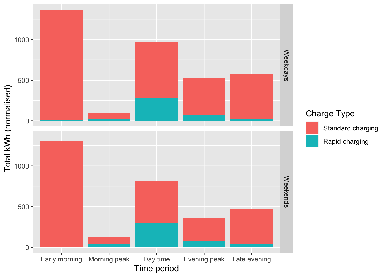
Figure 5.24: Total normalised kWh by weekday and charge type

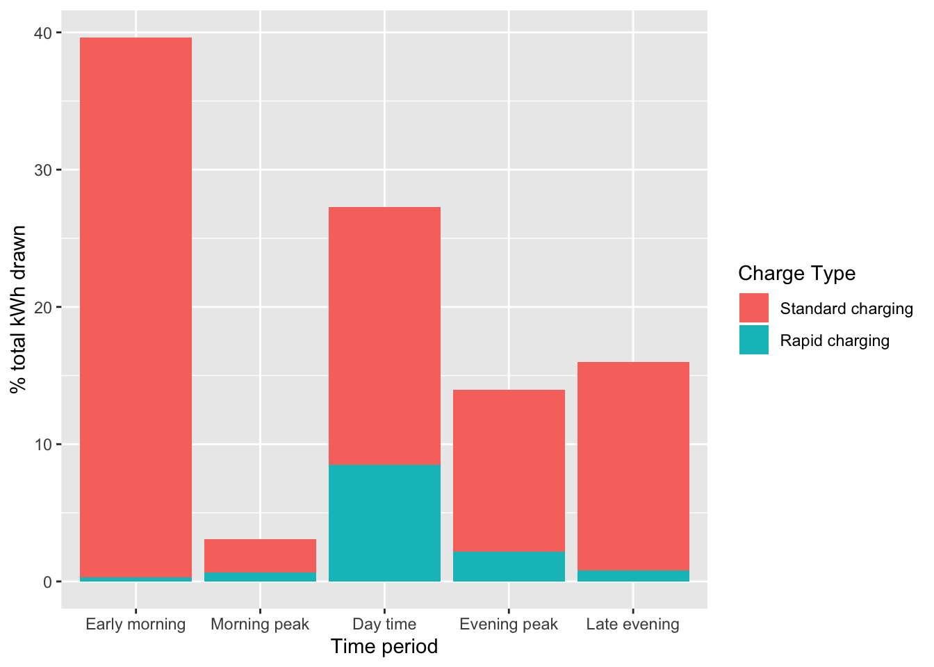
Figure 5.25: % total kWh by charge type and peak period

Table 5.12: Total kWh per period by charge type

Time period	Charge Type	Total kWh	% of total kWh
Early morning	Standard charging	9357.66	39.32
Morning peak	Standard charging	579.23	2.43
Day time	Standard charging	4466.36	18.77
Evening peak	Standard charging	2817.16	11.84
Late evening	Standard charging	3617.89	15.20
Early morning	Rapid charging	75.56	0.32
Morning peak	Rapid charging	159.92	0.67
Day time	Rapid charging	2026.08	8.51
Evening peak	Rapid charging	511.46	2.15
Late evening	Rapid charging	187.02	0.79

##           chargeType % of total kWh
## 1: Standard charging       87.56199
## 2:    Rapid charging       12.43801

##           chargeType Mean daily kWh where any charging   median      min      max
## 1: Standard charging                          8.111444 7.380983 0.008349 39.72797
## 2:    Rapid charging                         10.137124 6.767287 0.125158 84.97989

Table 5.12 and Figure 5.12 summarise the energy consumption across peak periods without weekday disaggregation. This shows that overall 55% of the energy drawn was overnight off-peak standard charging. Day time standard charging was 19% of the total and day-time rapid only 9%. Evening peak standard charging was 12% of total energy.

Overall, the EVs in this sample drew relatively little energy during the potentially problematic evening peak period.

6 Modelling the national electricity grid impact

Warning: we think this method is incorrect. Do not use results in this section. Yet.

If we make the heroic assumption that the future EV owners of Aotearoa will charge their vehicles in the same way and with the same temporal patterns as this small sample of early adopters then we can make estimates of the likely consequences for electricity demand under a range of scenarios using the data reported in Figure 5.6. This showed the mean % of EVs which were charging in each quarter-hour of the day by charge type.

Based on Table 4.5, we can repeat the process used in Section 5.6 by estimating:

• standard charging = 1.76 kW (median)
• rapid charging = 31.09 kW (median)

And that:

• there are 1,771,300 households in New Zealand (https://www.stats.govt.nz/information-releases/dwelling-and-household-estimates-june-2019-quarter)
• Car ownership 2013 (http://archive.stats.govt.nz/Census/2013-census/profile-and-summary-reports/quickstats-transport-comms/number-motor-vehicles.aspx):
  • 8% have no car
  • 37% have 1
  • 38% have 2
  • 16% have 3+ (we can treat this as 3)

We can now use the results shown in Figure 5.6 to construct a number of EV uptake scenarios such as:

• All households with >= 1 car switch one of them (or the one they have) to an EV (scenario 1) and their charging behaviour is exactly as reported in Figure 5.6

Using the very out of date Census 2013 data we can estimate that:

• we have 1,629,596 car owning households of which
  • 655,381 have 1 car
  • 673,094 have 2 cars
  • 283,408 have 3+ cars

We now apply the % charge rates calculated above to these values to estimate the additional power demand.

6.1 Scenario 1: All households with >= 1 car switch one of them (or the one they have) to an EV

Under this scenario (Figure 6.1) we can see demand increases by ~ 500 MW during the late evening and overnight due to standard charging which tends to avoid peak periods. On the other hand rapid charging, although less frequent (see Figure 5.6) has a bigger effect due to it’s larger power draw.

Figure 6.1: Estimated MW demand under scenario 1 (1 ICE <-> EV substitute for all households with cars)

Table 6.1: Estimated mean MW demand by charge type and period (Scenario 1)

peakPeriod	chargeType	Mean estimated MW
Early morning	Standard charging	527.69
Early morning	Rapid charging	1345.96
Morning peak	Standard charging	181.82
Morning peak	Rapid charging	1438.56
Day time	Standard charging	231.05
Day time	Rapid charging	1523.44
Evening peak	Standard charging	283.20
Evening peak	Rapid charging	1494.03
Late evening	Standard charging	483.83
Late evening	Rapid charging	1450.41

As we would expect this plot shows exactly the same distribution as Figure ??.

To determine whether this is a significant proportion of New Zealand national demand we convert the mean the MW values to MWh per half-hour for comparison with mean MWh per half-hour national generation values sourced from the EA’s EMI XX reference XXX.

6.1.1 Summer

Figure ?? shows the result of this calculation for the summer period. This uses wholesale generation data from January, February and December 2018 and the EV charging data for the study period as reported above. We assume that the EV charging behaviour is not seasonally affected although this may not necessarily be true in practice. Note that the rarity of rapid charging causes some zero values for this charge type.

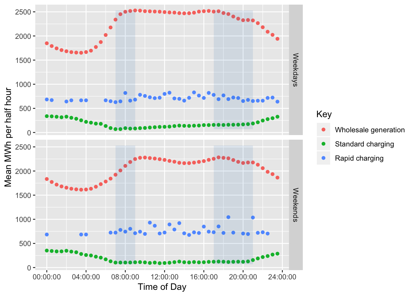
Figure 6.2: Actual wholesale generation and estimated energy consumption under Scenario 1 for the study period during the summer.

Table 6.2: Mean % of observed wholesale generation by peak period (summer)

weekdays	peakPeriod	meanRapidPC	meanStdPC
Weekdays	Early morning	21.13	14.34
Weekdays	Morning peak	28.04	3.16
Weekdays	Day time	29.82	4.96
Weekdays	Evening peak	29.42	6.71
Weekdays	Late evening	31.74	12.25
Weekends	Early morning	11.53	16.41
Weekends	Morning peak	37.11	5.07
Weekends	Day time	34.96	4.84
Weekends	Evening peak	30.55	5.43
Weekends	Late evening	25.40	11.31

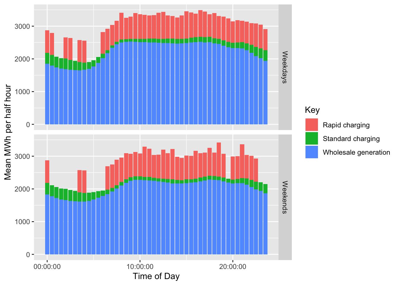
Figure 6.3: Actual wholesale generation and estimated energy consumption under Scenario 1 for the study period during the summer.

6.1.2 Winter

Figure ?? shows the result of this calculation for the summer period. This uses wholesale generation data from June, July and August 2018 and the EV charging data for the study period as reported above. as we do not have EV charging data for a winter period, we assume that the EV charging behaviour is not seasonally affected although this may not necessarily be true in practice. Note that the rarity of rapid charging causes some zero values for this charge type.

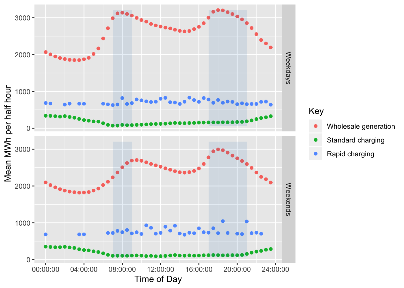
Figure 6.4: Actual wholesale generation and estimated energy consumption under Scenario 1 during the winter.

Table 6.3: Mean % of observed wholesale generation by peak period (winter)

weekdays	peakPeriod	meanRapidPC	meanStdPC
Weekdays	Early morning	18.53	12.72
Weekdays	Morning peak	22.27	2.51
Weekdays	Day time	26.78	4.48
Weekdays	Evening peak	22.97	5.24
Weekdays	Late evening	27.21	10.56
Weekends	Early morning	10.14	14.48
Weekends	Morning peak	31.40	4.29
Weekends	Day time	30.83	4.27
Weekends	Evening peak	23.85	4.24
Weekends	Late evening	21.84	9.90

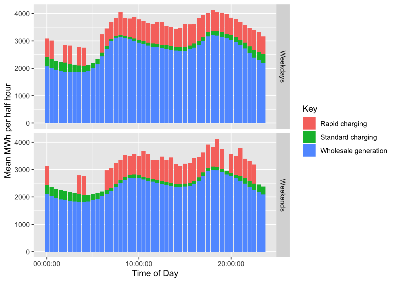
Figure 6.5: Actual wholesale generation and estimated energy consumption under Scenario 1 during the winter.

7 Summary

Based on a relatively small and probably non-representative sample of 48 domestic electric vehicles provided by our research partner FlipTheFleet and which were monitored from Inf to -Inf we have found that:

• Power supplied: The median power supplied during a charging event coded as ‘standard’ was 1.76 kW. The mean was slightly higher at 2.09 kW. Charging observations coded as ‘Rapid’ had a median of 1.76 kW (mean = 2.09 kW). Mean power when charging showed a complex temporal profile for weekday standard charging (Figure 5.17) with a peak of ~ 2.5kw at 10:00 and a second of the same value at around 18:00 with further peaks just after midnight. The inverse is seen on weekends with a charge peak during the middle of the day;
• Charging duration: Charging durations tended to fall into one of two groups. Longer ‘standard’ charges had a median duration of 207.12 minutes and a mean duration of 243.01 minutes. High power ‘Rapid’ charge events had a median duration of 14.26 minutes and a mean duration of 14.26 minutes;
• Time of day: Standard charging events tended to be the most frequent around 22:00 on both weekdays and weekends, suggesting the drivers in our dataset utilise timers to take advantage of off-peak electricity although this is not universal with a substantial proportion of charging events starting earlier in the day and potentially at higher power levels (see above). Rapid charging events tended to begin at 11:30am on weekdays and 1pm during weekends;
• State of charge: As has been previously shown (Speidel and Bräunl 2014), any drivers begin recharging with greater than 50% charge still remaining in the battery for both standard and rapid charge events. This has clear implications both for the management of battery life and also for the potential for vehicle-to-grid power flows during peak demand periods where vehicles may be at or arriving home with substantial available charge.

In the data provided for this study, most charging occurs at home using either a 1.8kw or 3kW charger, and commonly occurs both in the evening peak period and through the night. In addition, many vehicles begin charging with significant battery capacity remaining, providing them with the ability to provide vehicle to grid energy transfer should that technology become widely available.

These preliminary findings support recent modelling work (Concept Consulting 2018) that suggests that any negative effects electric vehicles may have on the evening national electricity grid peaks should be mitigatable through ‘smart’ charging methods. In addition, our analysis indicates that this may already be occurring to some extent in this sample of EV owners. If later adopters of electric vehicles can be induced to follow the same ‘smart’ charging patterns as those displayed in some of our data sample, it is likely that the effects that electric vehicles are otherwise likely to have on the electricity grid may be mitigated.

8 Statistical Annex

Data used:

• /Users/ben/Data/NZ_FlipTheFleet/processed/EVBB_processed_all_v2.0_20190604.csv.gz

If this is not what you expect this may be a test run using preliminary data.

8.1 Flip The Fleet data description

8.1.1 Raw data

Data description for original data supplied (before processing or filtering).

skimr::skim(rawDT)

Table 8.1: Data summary

Name	rawDT
Number of rows	1882040
Number of columns	9
_______________________
Column type frequency:
character	3
difftime	1
numeric	3
POSIXct	2
________________________
Group variables	None

Variable type: character

skim_variable	n_missing	complete_rate	min	max	empty	n_unique	whitespace
id	0	1	32	32	0	52	0
dvID	0	1	9	10	0	52	0
charging	0	1	26	31	0	2	0

Variable type: difftime

skim_variable	n_missing	complete_rate	min	max	median	n_unique
timeChr	0	1	0 secs	86399 secs	44877 secs	86400

Variable type: numeric

skim_variable	n_missing	complete_rate	mean	sd	p0	p25	p50	p75	p100	hist
charge_power_kw	0	1.00	1.59	63.73	0	0.00	1.30	1.85	74940.42	▇▁▁▁▁
state_of_charge_percent	0	1.00	69.00	20.66	0	56.31	70.41	83.05	1677.72	▇▁▁▁▁
odometer_km	1255614	0.33	7789.97	8268.44	-62920	2166.25	5309.00	11154.00	73607.00	▁▁▇▁▁

Variable type: POSIXct

skim_variable	n_missing	complete_rate	min	max	median	n_unique
r_dateTime	137	1	2018-04-05 10:34:41	2019-03-01 17:42:35	2018-11-25 21:21:08	1784161
r_dateTimeHalfHour	137	1	2018-04-05 10:30:00	2019-03-01 17:30:00	2018-11-25 21:00:00	12831

8.1.2 Processed and cleaned data

Data description for cleaned data (all observations).

skimr::skim(cleanDT)

Table 8.2: Data summary

Name	cleanDT
Number of rows	1074730
Number of columns	24
_______________________
Column type frequency:
character	4
Date	1
difftime	4
factor	3
numeric	6
POSIXct	6
________________________
Group variables	None

Variable type: character

skim_variable	n_missing	complete_rate	min	max	empty	n_unique	whitespace
id	0	1	32	32	0	48	0
dvID	0	1	9	10	0	48	0
weekdays	0	1	8	8	0	2	0
chargeFlag	2	1	17	25	0	5	0

Variable type: Date

skim_variable	n_missing	complete_rate	min	max	median	n_unique
date	0	1	2018-10-01	2019-01-16	2018-11-22	108

Variable type: difftime

skim_variable	n_missing	complete_rate	min	max	median	n_unique
timeChr	0	1	0 secs	86399 secs	43858 secs	86394
hms	0	1	0 secs	86399 secs	43858 secs	86394
qHour	0	1	0 secs	85500 secs	43200 secs	96
r_dateTimeDiff	14	1	0 secs	2486002 secs	50 secs	11447

Variable type: factor

skim_variable	n_missing	complete_rate	ordered	n_unique	top_counts
day_of_week	0	1	TRUE	7	Fri: 173053, Wed: 170267, Thu: 165276, Tue: 156780
chargeType	0	1	FALSE	3	Sta: 716907, Not: 350923, Rap: 6900
peakPeriod	0	1	FALSE	5	Ear: 356511, Day: 347804, Eve: 163020, Lat: 147782

Variable type: numeric

skim_variable	n_missing	complete_rate	mean	sd	p0	p25	p50	p75	p100	hist
charge_power_kw	0	1.0	1.59	2.87	0	0.0	1.47	1.92	70.16	▇▁▁▁▁
SoC_percent	41	1.0	68.81	18.58	0	56.1	70.21	82.89	98.10	▁▂▅▇▇
odometer_km	750182	0.3	7287.47	8339.26	-62920	1991.0	4752.00	9142.00	69394.00	▁▁▇▂▁
month	0	1.0	9.71	3.42	1	10.0	11.00	12.00	12.00	▁▁▁▁▇
odometerDiff	756512	0.3	1.59	2499.84	-64324	0.0	0.00	1.00	64261.00	▁▁▇▁▁
tempkW	0	1.0	0.20	2.66	0	0.0	0.00	0.00	70.16	▇▁▁▁▁

Variable type: POSIXct

skim_variable	n_missing	complete_rate	min	max	median	n_unique
r_dateTime	0	1	2018-10-01 13:00:10	2019-01-16 12:59:55	2018-11-22 12:00:37	1011415
startTime	0	1	2018-10-01 13:00:10	2019-01-16 12:59:55	2018-11-22 12:00:37	1011415
r_dateTimeHalfHour	0	1	2018-10-01 13:00:00	2019-01-16 12:30:00	2018-11-22 12:00:00	5135
r_dateTimeQhour	0	1	2018-10-01 13:00:00	2019-01-16 12:45:00	2018-11-22 12:00:00	10253
r_dateTime1MinFl	0	1	2018-10-01 13:00:00	2019-01-16 12:59:00	2018-11-22 12:00:00	152837
r_dateTime1MinR	0	1	2018-10-01 13:00:00	2019-01-16 13:00:00	2018-11-22 12:00:30	152843

Data description for cleaned data (first observations in a charging sequence).

skimr::skim(firstCleanDT)

Table 8.3: Data summary

Name	firstCleanDT
Number of rows	2986
Number of columns	24
_______________________
Column type frequency:
character	5
Date	1
difftime	6
factor	5
numeric	5
POSIXct	2
________________________
Group variables	None

Variable type: character

skim_variable	n_missing	complete_rate	min	max	empty	n_unique	whitespace
id	0	1	32	32	0	48	0
dvID	0	1	9	10	0	48	0
weekdays	0	1	8	8	0	2	0
chargeFlag	0	1	25	25	0	1	0
chargeTypeError	0	1	31	37	0	4	0

Variable type: Date

skim_variable	n_missing	complete_rate	min	max	median	n_unique
date	0	1	2018-10-01	2019-01-16	2018-11-22	108

Variable type: difftime

skim_variable	n_missing	complete_rate	min	max	median	n_unique
timeChr	0	1	40 secs	86246 secs	56268.0 secs	2871
hms	0	1	40 secs	86246 secs	56268.0 secs	2871
qHour	0	1	0 secs	85500 secs	55800.0 secs	96
r_dateTimeDiff	0	1	0 secs	230025 secs	339.0 secs	1685
endTime	0	1	31 secs	86342 secs	40739.5 secs	2921
pairDuration	0	1	1 secs	97003 secs	10904.0 secs	2752

Variable type: factor

skim_variable	n_missing	complete_rate	ordered	n_unique	top_counts
day_of_week	0	1	TRUE	7	Fri: 474, Wed: 451, Mon: 445, Thu: 443
chargeType	0	1	FALSE	2	Sta: 2607, Rap: 379, Not: 0
peakPeriod	0	1	FALSE	5	Day: 1147, Lat: 699, Eve: 556, Ear: 408
endType	0	1	FALSE	2	Sta: 2664, Rap: 322, Not: 0
chargeTypeCorrected	0	1	FALSE	2	Sta: 2594, Rap: 392, Not: 0

Variable type: numeric

skim_variable	n_missing	complete_rate	mean	sd	p0	p25	p50	p75	p100	hist
charge_power_kw	0	1.00	6.73	12.14	0.50	1.56	2.08	3.30	70.16	▇▁▁▁▁
SoC_percent	0	1.00	50.28	19.22	4.11	36.28	49.02	60.92	98.10	▁▆▇▃▂
odometer_km	2367	0.21	6641.21	7567.25	-52352.00	1775.00	4342.00	9440.00	38453.00	▁▁▃▇▁
month	0	1.00	9.56	3.58	1.00	10.00	11.00	12.00	12.00	▂▁▁▁▇
odometerDiff	2382	0.20	54.21	2410.82	-18760.00	0.00	0.00	0.00	37626.00	▁▇▁▁▁

Variable type: POSIXct

skim_variable	n_missing	complete_rate	min	max	median	n_unique
r_dateTime	0	1	2018-10-01 13:27:27	2019-01-16 12:33:43	2018-11-22 21:33:13	2986
startTime	0	1	2018-10-01 13:27:27	2019-01-16 12:33:43	2018-11-22 21:33:13	2986

8.2 Odometer data checks

There are many NAs in the odometer data and also -ve values as Table 8.4 shows. Given the apparently poor quality of the data we do not use odometer data in this report.

rawDT[odometer_km < 0, odometerFlag := "-ve" ]
rawDT[odometer_km == 0, odometerFlag := "0" ]
rawDT[odometer_km > 0, odometerFlag := "+ve" ]

t <- with(rawDT, table(id,
     odometerFlag, useNA = "always"))

kableExtra::kable(t, caption = "Count of -ve, 0, +ve and NA odometer readings by vehicle (original data)") %>%
  kable_styling()

Table 8.4: Count of -ve, 0, +ve and NA odometer readings by vehicle (original data)

	-ve	+ve	0	NA
009e8a24229d1c7723588ceec2b95f6a	186	82476	0	2537
0155fb80d2ef801d7086a159c5fe8df0	11	7876	3	32998
01583b8a5f0344cc4aa3b3939a27af2a	4	0	0	0
0564346e7607d1c21e5a6e3878399307	40	15940	2	39263
0af7e964b7e72ab184fbead5d30106e3	22	10751	5	77445
0cc746a3f5ae75ee94068a8354b6be08	0	3	0	0
1256011bed883244df94d560795904e8	310	33783	0	1364
126c8759ec95ba40070b16a11fe0e587	3	0	0	255
12f1e87977249e72358c12dcd197f753	153	16504	1	50609
16b47e88aec68658c5f03db9546db91b	2	2711	2	4185
19c4d7520e9d65c364ff0729a7caf426	117	12847	1	480
1c43f265e57e648c89a427add181e58f	73	16525	0	47822
2f1aeb0d0c5d7a823533b8633d808332	4	3230	4	6707
32346e168dbccf81c465ed657e5fc371	76	19917	17	50582
3993011700868644dc948d58dd3bf9d7	93	3494	9	11768
3aa51bc2789088cf6a3804c50f362f34	4	11685	1	50299
3c218d73c404cc8a552f3449b64f403a	19	3204	47	4097
3dfd17f381f439bc351065cff0d83c69	851	21524	1	54441
3fcc39331391ecd9280917d6bdf321bb	414	14609	2	34223
41930b96d7e6cc4a5eb6542ca36f09e2	0	5256	3	11877
49be6e824b8a4196cc514c2ce4cb6e68	296	31792	0	26927
4a6bb6e7ffc28d9d8eda7b4c6377a027	16	3	0	0
4e48f4155c29c763ffe6d9e17a495200	79	1854	2	4338
5580d13143df1b944fdc1d89ec402b8e	175	20005	15	37670
5bf3a96857982acaa939fd1adc988e07	0	5745	4	9862
5ddc10f96e80630519747ba6a8fe682f	1	9631	1	80
60593731dff536355c4bd88c1c1e5cdb	103	5100	4	14445
616cde60ad25ddc1db4dd832ff1231ca	126	6782	2	33292
6e3293c77f562262ed6608db1b596d36	0	4288	0	27
70102a8511c6454814b7ca1506d461dd	33	5308	45	12491
7023838bd3a5004be2d10784bc116d54	0	1619	1	6974
746039182479252e9d1c9eeb071695ec	349	11902	2	23483
781f06f7d7bb80b74c399326be0d3e28	419	1419	14	3617
7c234b2fb2fc9db5a1a1321167606eba	97	29619	1	69761
80160eb40e4f12004b46d4cf77dcd62f	131	21159	2	117518
8a217a62f385a9c6698033b38b169d70	97	28408	0	1541
8ccb51191dcf0dd9152b867f6e1f74d4	176	3970	1	20941
8d4a65c57c5d778786189f96df2c65c5	227	9130	2	15644
9447d58925397798b076e4b5bf42fd43	9	5829	5	18892
a1c8e57bfcf815f25844c49f4535a8ef	4	7832	2	27540
bb1a2db7ae160eba9d77bb7c35c57f05	2	8931	3	32765
bc3bd38c67b3b2cb2757c94b54a5b408	36	7147	0	9816
bdbbb99fdb70e1e108bb69eff77ee48a	141	24744	2	65667
c05b76de4b11ef7ec0c84e6dc3d05f9c	16	14598	339	52110
da5dcd6efbca045af6759f645f51b6a0	137	9617	2	24606
e11e3f82945d94d288a7e47c06515f26	26	7558	1	38693
f616ac16a4a9af35eacd2afa9a98f7f1	19	10146	3	31736
f8afdd8b06b89cfcfadd75f5146736cd	44	14552	0	1678
f99c233aec9005793d82e64afb45aa23	41	4637	3	10469
fc6a67af46efb8ab97e2e014173af954	128	11862	5	46543
fc9cb5463304eb870e70f6720185d653	0	6646	1	6942
fd60aa4d6f3748b3f36495ff1a823407	0	6383	5	8594
NA	0	0	0	0

8.3 Coding checks

8.3.1 Charge flag

This is used to identify observations that form part of a sequence. The logic is given in Section 4.3.2. Here we show the results of applying an additional 120 second rule. In this case a sequence only exists where we have charging observations which have less than 120 seconds between them.

kableExtra::kable(sequenceMethod1_T, caption = "Charge sequence flags (120 second rule)") %>%
  kable_styling()

Table 8.5: Charge sequence flags (120 second rule)

	Standard charging	Rapid charging	Not charging	NA
Charging in a seq	1015390	11896	0	0
First charge obs in a seq	7540	562	0	0
Last charge in a seq	10351	644	0	0
Not charging (0 kW)	0	0	805358	0
Not classified (what is this??)	20359	673	0	0
Single charge observation	8593	391	0	0
NA	230	53	0	0

kableExtra::kable(sequenceMethod2_T, caption = "Charge sequence flags (no 120 second rule)") %>%
  kable_styling()

Table 8.5: Charge sequence flags (no 120 second rule)

	Standard charging	Rapid charging	Not charging	NA
Charging in a seq	1032720	12291	0	0
First charge obs in a seq	10454	816	0	0
Last charge in a seq	10609	670	0	0
Not charging (0 kW)	0	0	805358	0
Single charge observation	8593	391	0	0
NA	87	51	0	0

As we can see, applying the 120 second rule reduces the number of observations categorised as part of a sequence as it will not know what to do with:

• charge -> gap of > 120 secs -> charge 120 secs -> charge

For now we therefore do not use the 120 second rule.

# Check chargeFlag ----
message("chargeFlag is used to classify charging events - check against charge type:")

## chargeFlag is used to classify charging events - check against charge type:

t <- table(cleanDT$chargeFlag, cleanDT$chargeType, useNA = "always")
kableExtra::kable(t, caption = "chargeFlag errors (clean data)") %>%
  kable_styling()

Table 8.6: chargeFlag errors (clean data)

	Standard charging	Rapid charging	Not charging	NA
Charging in a seq	699162	6093	0	0
First charge obs in a seq	6519	381	0	0
Last charge in a seq	6575	323	0	0
Not charging (0 kW)	0	0	350923	0
Single charge observation	4650	102	0	0
NA	1	1	0	0

message("There are a few observations that have chargeFlag = NA but are charging... why?")

## There are a few observations that have chargeFlag = NA but are charging... why?

We also test the patterns of charging that this classification produces. We do this first for ‘standard’ charging sequences and then for ‘Rapid’ charging sequences.

# debug sequences visually ----

# start & end charge rate ----
firstLastDT <- firstLastDT[, startChargekW := charge_power_kw]
firstLastDT <- firstLastDT[, endChargekW := shift(charge_power_kw, type = "lead")]

# start & end batter state
firstLastDT <- firstLastDT[, startSoC_pc := SoC_percent]
firstLastDT <- firstLastDT[, endSoC_pc := shift(SoC_percent, type = "lead")]

# calc duration so we can decide what to do where it is -ve - i.e. event spanned midnight ----
firstLastDT <- firstLastDT[, notDuration := difftime(endTime, startTime, units='mins'), by = id] # set all within id, if this is -ve then it spanned midnight
# fix # 1
firstLastDT <- firstLastDT[, endTimeTrunc := ifelse(notDuration < 0, 
                                                   hms::parse_hm("23:59"),
                                                   endTime)] # this truncates charge periods that span midnight and ends then at midnight for clarity. Of course this makes a hash of early morning charging patterns... 

# charge rate & state of charge deltas ----
firstLastDT <- firstLastDT[, chargePowerDelta := endChargekW - charge_power_kw] # should be -ve where we start high and end low
firstLastDT <- firstLastDT[, SoC_pcDelta := endSoC_pc - startSoC_pc] # should be -ve where we start high and end low

Figure 8.1 plots the first and last charge observation in a sequence for all pairs and for all vehicles where events were classified as (corrected) ‘standard’ charges. The y value is charging rate (kW) at the start and end of the sequence. Colour (red end of the scale) is used to highlight pairs which show an ‘odd’ pattern - e.g. the charge rate increased.

# format labels function
# https://stackoverflow.com/questions/53804629/how-to-format-difftime-as-hhmm-in-ggplot2
format_hm <- function(sec) stringr::str_sub(format(sec), end = -4L)
# plotting function
makeSeqChargePlot <- function(dt, y = y, yend = yend, colour = colour){
  p <- ggplot2::ggplot(dt) +
    geom_segment(aes(x = hms::as.hms(startTime), # start x value
                     xend = hms::as.hms(endTimeTrunc), # end x value
                     y = get(y), # start y value
                     yend = get(yend), # end y value
                     colour = get(colour))) + # colour to highlight some value
    labs(x = "Sequence start and end time") + 
    theme(legend.position = "bottom") +
    scale_x_time(labels = format_hm) +
    facet_wrap(. ~ dvID)
  return(p)
}

dt <- firstLastDT[chargeTypeCorrected %like% "Standard" & 
                    #startChargekW < 5 & #use this to filter out the few that seem to have 6kW chargers (they could also be mis-coded 'Rapid' charging)
                    chargeFlag %like% "First"]

p <- makeSeqChargePlot(dt, y = "startChargekW", 
                       yend = "endChargekW", 
                       colour =  "chargePowerDelta") 
p <- p + 
  labs(y = "Charging rate (kW)",
       caption = "Standard charging (corrected) \n 
       Pairs spanning midnight truncated at 23:59 \n
       Peak periods shaded") +
  guides(colour = guide_legend(title = "Charge rate delta (kW)")) +
  scale_color_continuous(low = "green", high = "red") # highlight ones that went up
yMin <- min(dt$startChargekW) # might not quite work if end is higher...
yMax <- max(dt$startChargekW) # might not quite work if end is higher...
addPeaks(p)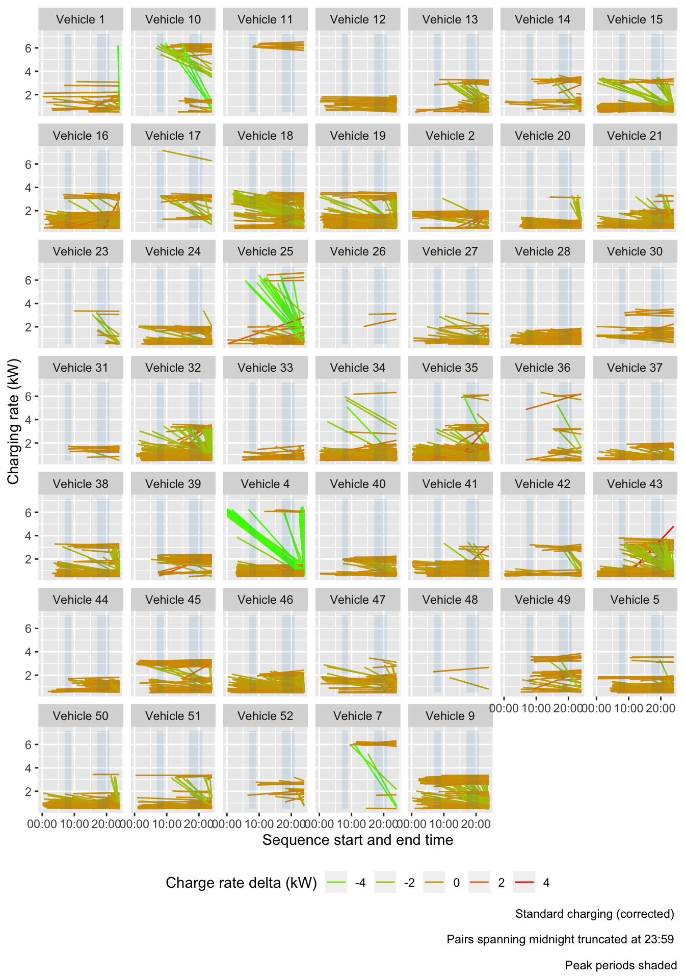

Figure 8.1: Standard charging (corrected) - rate of charge

#ggsave("plots/standardChargePairs_kW_LineSegments.png", p, height = 10)

Figure 8.2 shows the distribution of charge power deltas by peak/not peak period (of start time) for ‘standard’ charge events. This suggests that the majority of charging events either hold power constant or decline over time with some sort of shoulder effect. A few increase. More of those which start in the ‘evening’ and ‘not peak’ period seem to hold the power level constant, presumably because the battery capacity is slightly lower at this time following day-time use.

p <- ggplot2::ggplot(dt, aes(x = chargePowerDelta, colour = peakPeriod)) +
  geom_density(alpha = 0.5) +
  guides(colour = guide_legend(title = "Peak period:")) +
  labs(x = "Change in power from start to end (kW)")
p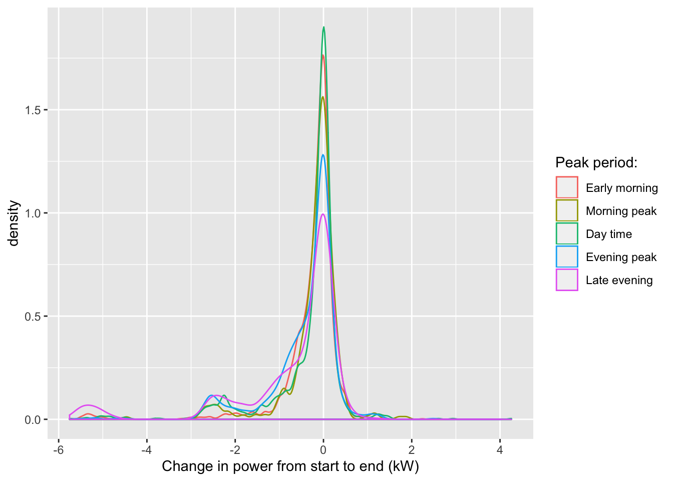

Figure 8.2: Histogram of charge power deltas by peak/not peak period

Figure 8.3 uses the same approach but in this case the y value is charging rate (kW) at the start and end of the sequence. Colour (red end of the scale) is used to highlight pairs which show an ‘odd’ pattern - e.g. the battery state of charge decreased.

#dt <- dt[, SoC_pcDelta := SoC_pcDelta * -1] # invert so big drops become red in plot
p <- makeSeqChargePlot(dt, y = "startSoC_pc", 
                       yend = "endSoC_pc", 
                       colour =  "SoC_pcDelta")
p <- p + 
  labs(y = "State of charge (%)",
       caption = "Standard charging (corrected) \n Pairs spanning midnight truncated at 23:59") +
  guides(colour = guide_legend(title = "State of charge delta (%)")) +
  scale_color_continuous(low = "red", high = "green") # highlight ones that went down
yMin <- min(dt$startSoC_pc) # might not quite work if end is higher...
yMax <- max(dt$startSoC_pc) # might not quite work if end is higher...
addPeaks(p)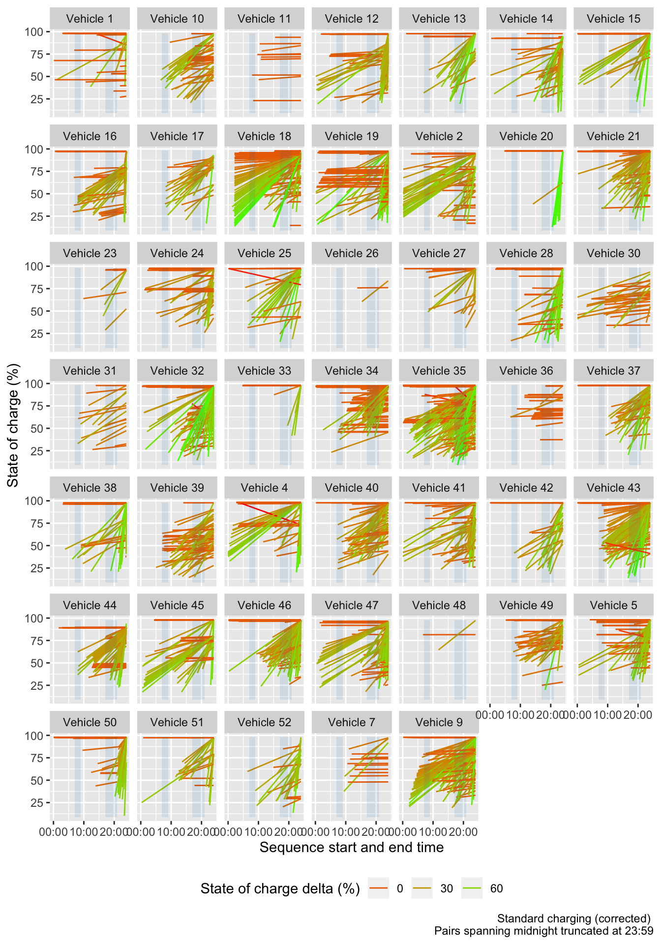

Figure 8.3: Standard charging (corrected) - state of charge

#ggsave("plots/standardChargePairs_SoC_LineSegments.png", p, height = 10)

Figure 8.4 and Figure 8.5 repeat these plots but for (corrected) ‘Rapid’ charge events.

dt <- firstLastDT[chargeTypeCorrected %like% "Rapid" & 
                    #startChargekW < 5 & #use this to filter out the few that seem to have 6kW chargers (or they might be 'Rapid' charging too)
                    chargeFlag %like% "First"]

p <- makeSeqChargePlot(dt, y = "startChargekW", 
                       yend = "endChargekW", 
                       colour =  "chargePowerDelta") 
p <- p + 
  labs(y = "Charging rate (kW)",
       caption = "Rapid charging (corrected) \n Pairs spanning midnight truncated at 23:59") +
  guides(colour = guide_legend(title = "Charge rate delta (kW)")) +
  scale_color_continuous(low = "green", high = "red") # highlight ones that went up
yMin <- min(dt$startChargekW) # might not quite work if end is higher...
yMax <- max(dt$startChargekW) # might not quite work if end is higher...
addPeaks(p)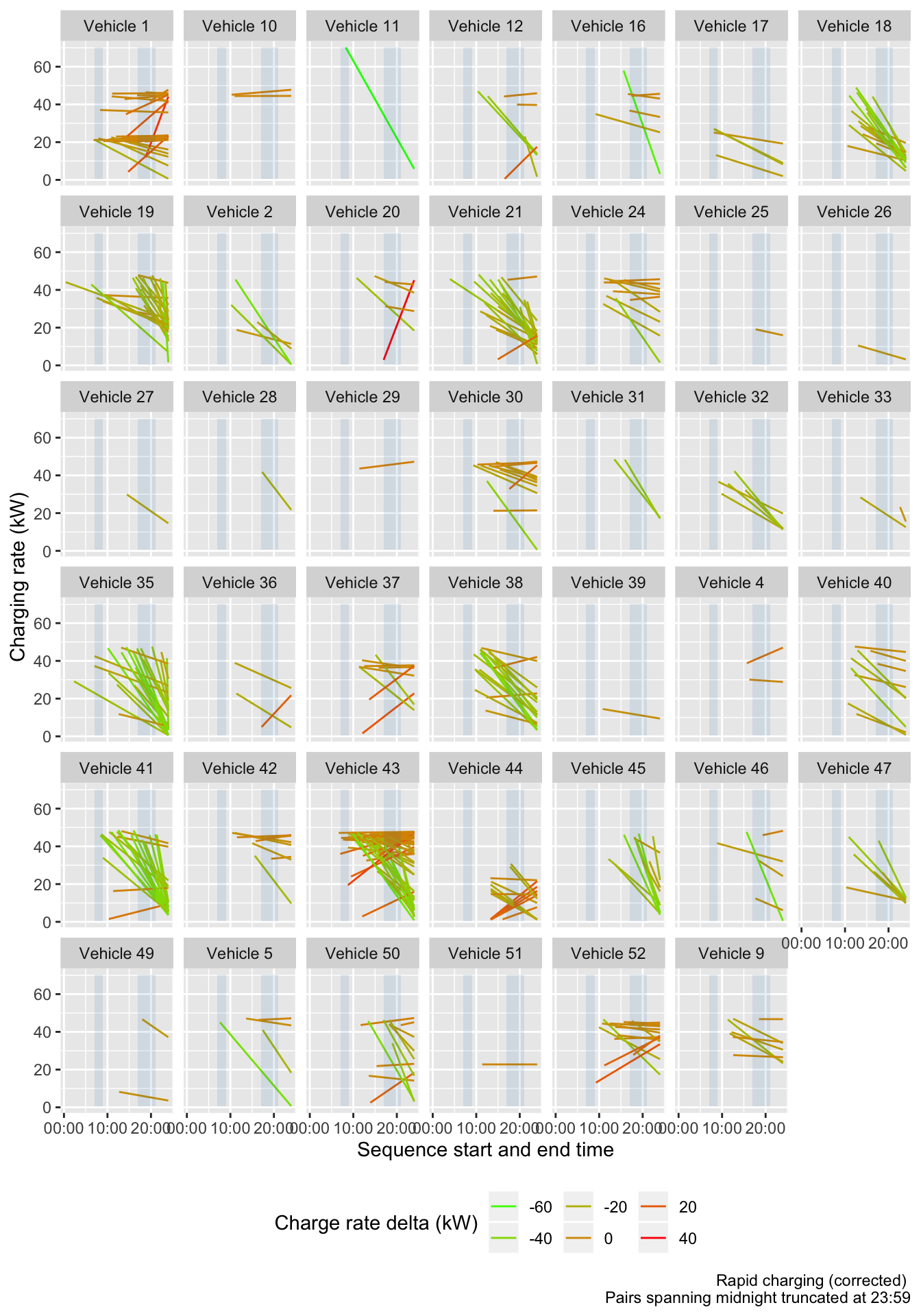

Figure 8.4: Rapid charging (corrected) - rate of charge

#ggsave("plots/RapidChargePairs_kW_LineSegments.png", p, height = 10)

#dt <- dt[, SoC_pcDelta := SoC_pcDelta * -1] # invert so big drops become red in plot
p <- makeSeqChargePlot(dt, y = "startSoC_pc", 
                       yend = "endSoC_pc", 
                       colour =  "SoC_pcDelta")
p <- p + 
  labs(y = "State of charge (%)",
       caption = "Rapid charging (corrected) \n Pairs spanning midnight truncated at 23:59") +
  guides(colour = guide_legend(title = "State of charge delta (%)")) +
  scale_color_continuous(low = "red", high = "green") # highlight ones that went down
yMin <- min(dt$startSoC_pc) # might not quite work if end is higher...
yMax <- max(dt$startSoC_pc) # might not quite work if end is higher...
addPeaks(p)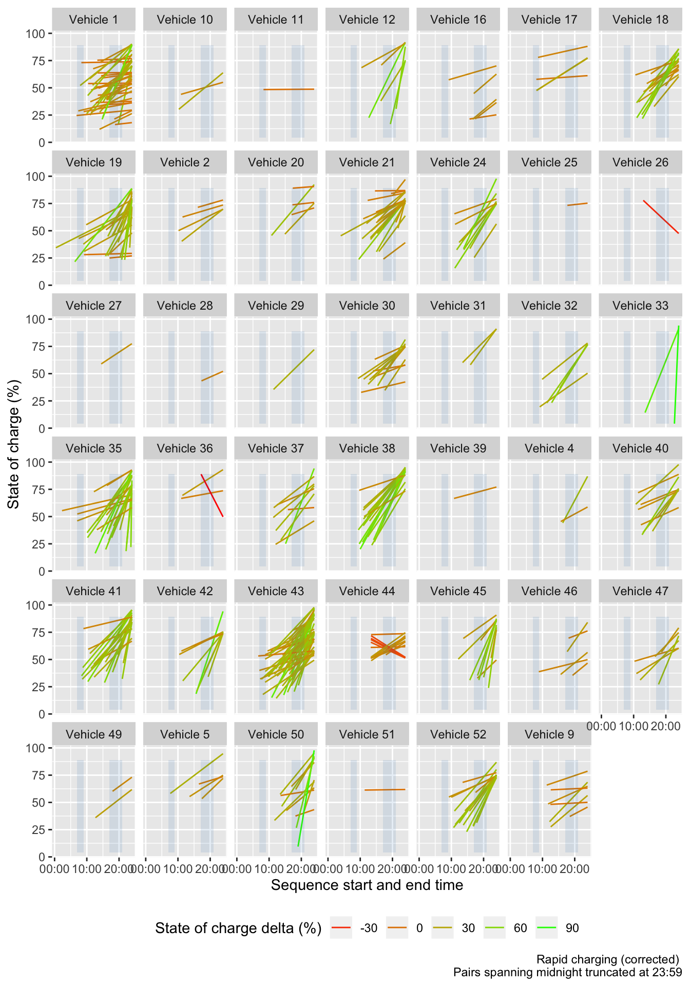

Figure 8.5: Rapid charging (corrected) - state of charge

#ggsave("plots/RapidChargePairs_SoC_LineSegments.png", p, height = 10)

Figure 8.6 shows the distribution of charge power deltas by peak/not peak period (of start time) for all ‘Rapid’ charge events. These show a rather different pattern.

p <- ggplot2::ggplot(dt, aes(x = chargePowerDelta, colour = peakPeriod)) +
  geom_density(alpha = 0.5) +
  guides(colour = guide_legend(title = "Peak period:")) +
  labs(x = "Change in power from start to end (kW)")
p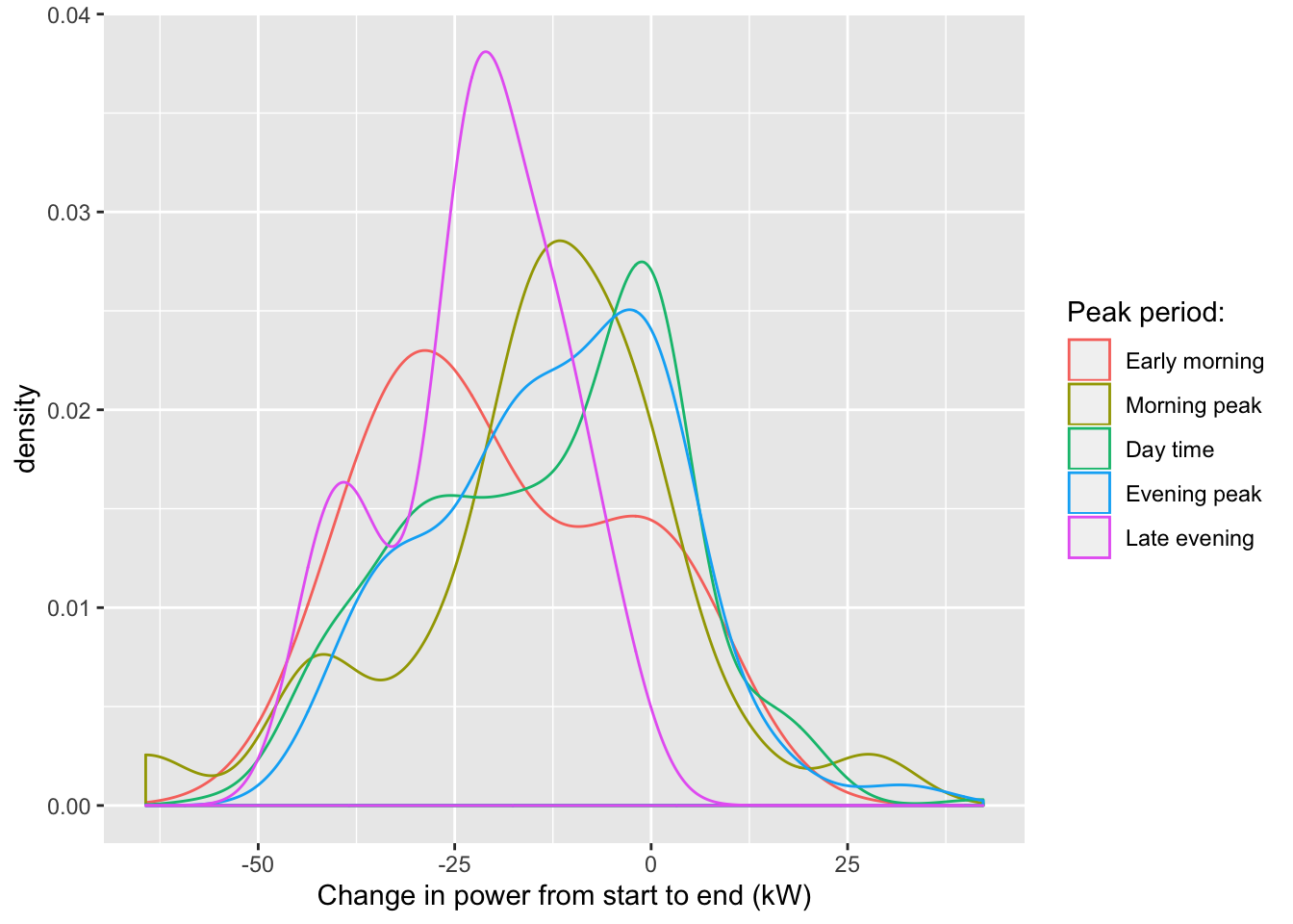

Figure 8.6: Histogram of charge power deltas by peak/not peak period

8.3.2 Charge type

chargeType is used to classify charging events into standard vs rapid using the 7 kW threshold. But there may be mis-classifications where a sequence starts on a rapid charger but power demand declines below the threshold. We can check this and have corrected it in some sections above using the start/end pairs.

# Check chargeType ----

t <- table(firstLastDT$chargeTypeError, firstLastDT$chargeType, useNA = "always")

kableExtra::kable(t, caption = "chargeType errors detected") %>%
  kable_styling()

Table 8.7: chargeType errors detected

	Standard charging	Rapid charging	Not charging	NA
Error: first = Rapid, last = Standard	0	72	0	0
Error: first = Standard, last = Rapid	14	0	0	0
OK: first = Rapid, last = Rapid	0	309	0	0
OK: first = Standard, last = Standard	6505	0	0	0
NA	6575	323	0	0

nError <- nrow(firstLastDT[chargeTypeError %like% "Error"])
nErrorEVs <- uniqueN(firstLastDT[chargeTypeError %like% "Error"]$dvID)  
message("There are ", nError, " pairs (out of a total of ", nrow(firstLastDT)/2,") from ", nErrorEVs ," EVs where charge type doesn't match.")

## There are 86 pairs (out of a total of 6899) from 26 EVs where charge type doesn't match.

References

Azadfar, Elham, Victor Sreeram, and David Harries. 2015. “The investigation of the major factors influencing plug-in electric vehicle driving patterns and charging behaviour.” Renewable and Sustainable Energy Reviews 42. Elsevier: 1065–76. https://doi.org/10.1016/j.rser.2014.10.058.

Concept Consulting. 2018. “‘ Driving change ’ – Issues and options to maximise the opportunities from large-scale electric vehicle uptake in New Zealand,” no. March.

Eyers, Lisa. 2018. “Electric Chargepoint Analysis 2017 : Domestics Key findings :” no. December.

Khan, Imran, Michael W. Jack, and Janet Stephenson. 2018. “Analysis of greenhouse gas emissions in electricity systems using time-varying carbon intensity.” Journal of Cleaner Production 184. Elsevier Ltd: 1091–1101. https://doi.org/10.1016/j.jclepro.2018.02.309.

Langbroek, Joram H. M., Joel P. Franklin, and Yusak O. Susilo. 2017. “When Do You Charge Your Electric Vehicle? A Stated Adaptation Approach.” Energy Policy 108 (September): 565–73. https://doi.org/10.1016/j.enpol.2017.06.023.

Li, Wenbo, Ruyin Long, Hong Chen, and Jichao Geng. 2017. “A Review of Factors Influencing Consumer Intentions to Adopt Battery Electric Vehicles.” Renewable and Sustainable Energy Reviews 78 (October): 318–28. https://doi.org/10.1016/j.rser.2017.04.076.

Rezvani, Zeinab, Johan Jansson, and Jan Bodin. 2015. “Advances in Consumer Electric Vehicle Adoption Research: A Review and Research Agenda.” Transportation Research Part D: Transport and Environment 34 (January): 122–36. https://doi.org/10.1016/j.trd.2014.10.010.

Speidel, Stuart, and Thomas Bräunl. 2014. “Driving and Charging Patterns of Electric Vehicles for Energy Usage.” Renewable and Sustainable Energy Reviews 40 (December): 97–110. https://doi.org/10.1016/j.rser.2014.07.177.

Stephenson, Janet, Rebecca Ford, Nirmal-Kumar Nair, Neville Watson, Alan Wood, and Allan Miller. 2017. “Smart grid research in New Zealand – A review from the GREEN Grid research programme.” https://doi.org/10.1016/j.rser.2017.07.010.

Transpower New Zealand. 2015. “Transmission Planning Report,” no. July: 320.

———. 2017. “Battery Storage in New Zealand,” no. September: 41. https://www.transpower.co.nz/sites/default/files/publications/resources/Battery Storage in New Zealand.pdf.