Otago University Medical School Buildings Energy Consumption Data
Ben Anderson (b.anderson@soton.ac.uk, @dataknut), Carsten Dortans (carsten.dortans@web.de)
Last run at: 2019-06-12 15:35:23
1 Setup
2 Load data
Use data.table::fread() to load the data. It deals with the ; delimiter automatically.
Loadng data from ~/Data/OtagoUni/MedicalSchoolBuildings.csv, reporting any warnings and listing the columns/variables:
rdt <- data.table::fread(path.expand(dFile),
                  )
## Warning in data.table::fread(path.expand(dFile), ): Detected 24 column
## names but the data has 21 columns. Filling rows automatically. Set
## fill=TRUE explicitly to avoid this warning.message("N rows:", nrow(rdt))## N rows:14337names(rdt)## [1] "Number"
## [2] "Time"
## [3] "Consumed Active Energy Total Tariff Sum L1-L3 (15m) [D206 Hercus]-avg[Wh]"
## [4] "Consumed Active Energy Total Tariff Sum L1-L3 (15m) [D206 Hercus]-min[Wh]"
## [5] "Consumed Active Energy Total Tariff Sum L1-L3 (15m) [D206 Hercus]-max[Wh]"
## [6] "Consumed Active Energy Total Tariff Sum L1-L3 (15m) [D201 and D203 Adams Sayer]-avg[Wh]"
## [7] "Consumed Active Energy Total Tariff Sum L1-L3 (15m) [D201 and D203 Adams Sayer]-min[Wh]"
## [8] "Consumed Active Energy Total Tariff Sum L1-L3 (15m) [D201 and D203 Adams Sayer]-max[Wh]"
## [9] "Consumed Active Energy Total Tariff Sum L1-L3 (15m) [D205 Scott]-avg[Wh]"
## [10] "Consumed Active Energy Total Tariff Sum L1-L3 (15m) [D205 Scott]-min[Wh]"
## [11] "Consumed Active Energy Total Tariff Sum L1-L3 (15m) [D205 Scott]-max[Wh]"
## [12] "Consumed Active Energy Total Tariff Sum L1-L3 (15m) [D204 LFB]-avg[Wh]"
## [13] "Consumed Active Energy Total Tariff Sum L1-L3 (15m) [D204 LFB]-min[Wh]"
## [14] "Consumed Active Energy Total Tariff Sum L1-L3 (15m) [D204 LFB]-max[Wh]"
## [15] "Consumed Active Energy Total Tariff Sum L1-L3 (15m) [D202 Wellcome]-avg[Wh]"
## [16] "Consumed Active Energy Total Tariff Sum L1-L3 (15m) [D202 Wellcome]-min[Wh]"
## [17] "Consumed Active Energy Total Tariff Sum L1-L3 (15m) [D202 Wellcome]-max[Wh]"
## [18] "Consumed Active Energy Total Tariff Sum L1-L3 (15m) [D20X Whole Medical School]-avg[Wh]"
## [19] "Consumed Active Energy Total Tariff Sum L1-L3 (15m) [D20X Whole Medical School]-min[Wh]"
## [20] "Consumed Active Energy Total Tariff Sum L1-L3 (15m) [D20X Whole Medical School]-max[Wh]"
## [21] "Active Energy Total Tariff Sum L1-L3 (30m) [D207 Generator]-avg[Wh]"
## [22] "Active Energy Total Tariff Sum L1-L3 (30m) [D207 Generator]-min[Wh]"
## [23] "Active Energy Total Tariff Sum L1-L3 (30m) [D207 Generator]-max[Wh]"
## [24] "V24"3 Clean and process original data
Keep the vars we want and test.
# keep the vars we want

cleanDT <- rdt[, .(Time,
                  avg = `Consumed Active Energy Total Tariff Sum L1-L3 (15m) [D20X Whole Medical School]-avg[Wh]`,
                  min = `Consumed Active Energy Total Tariff Sum L1-L3 (15m) [D20X Whole Medical School]-min[Wh]`,
                  max = `Consumed Active Energy Total Tariff Sum L1-L3 (15m) [D20X Whole Medical School]-max[Wh]`)]

message("Keeping: ")
## Keeping:names(cleanDT)## [1] "Time" "avg" "min" "max"Now clean the data. During this process we force R to think the timezone of the original Time variable is NZ Time. If we didn’t R might (sometimes) assume it is UTC and we would then get DST break errors and incorrect daily profiles.
cleanDT[, dateTime := lubridate::dmy_hms(Time)] # is this UTC? No we think it's NZ time
cleanDT[, dateTime := lubridate::force_tz(dateTime, tzone = "Pacific/Auckland")]
cleanDT[, hour := lubridate::hour(dateTime)]

cleanDT[, hms := hms::as.hms(dateTime)]
cleanDT[, date := lubridate::date(dateTime)]
cleanDT[, dow := lubridate::wday(date, label = TRUE)]
cleanDT[, month := lubridate::month(date, label = TRUE)]

# check
t <- head(cleanDT[, .(Time, dateTime, hour)])

kableExtra::kable(t, caption = "Testing conversion of Time variable")| Time | dateTime | hour |
|---|---|---|
| 1/01/19 12:15:00 AM | 2019-01-01 00:15:00 | 0 |
| 1/01/19 12:30:00 AM | 2019-01-01 00:30:00 | 0 |
| 1/01/19 12:45:00 AM | 2019-01-01 00:45:00 | 0 |
| 1/01/19 1:00:00 AM | 2019-01-01 01:00:00 | 1 |
| 1/01/19 1:15:00 AM | 2019-01-01 01:15:00 | 1 |
| 1/01/19 1:30:00 AM | 2019-01-01 01:30:00 | 1 |
Now summarise and test consumption.
s <- summary(cleanDT)

kableExtra::kable(s, caption = "Summary of data") %>%
kable_styling()| Time | avg | min | max | dateTime | hour | hms | date | dow | month | |
|---|---|---|---|---|---|---|---|---|---|---|
| Length:14337 | Min. :2.767e+10 | Min. :2.767e+10 | Min. :2.767e+10 | Min. :2019-01-01 00:15:00 | Min. : 0.00 | Length:14337 | Min. :2019-01-01 | Sun:2014 | Mar :2976 | |
| Class :character | 1st Qu.:2.811e+10 | 1st Qu.:2.811e+10 | 1st Qu.:2.811e+10 | 1st Qu.:2019-02-07 08:15:00 | 1st Qu.: 5.00 | Class1:hms | 1st Qu.:2019-02-07 | Mon:2009 | Jan :2975 | |
| Mode :character | Median :2.860e+10 | Median :2.860e+10 | Median :2.860e+10 | Median :2019-03-16 18:30:00 | Median :11.00 | Class2:difftime | Median :2019-03-16 | Tue:2111 | Apr :2880 | |
| NA | Mean :2.861e+10 | Mean :2.861e+10 | Mean :2.861e+10 | Mean :2019-03-16 18:08:04 | Mean :11.48 | Mode :numeric | Mean :2019-03-16 | Wed:2112 | May :2827 | |
| NA | 3rd Qu.:2.910e+10 | 3rd Qu.:2.910e+10 | 3rd Qu.:2.910e+10 | 3rd Qu.:2019-04-23 02:30:00 | 3rd Qu.:17.00 | NA | 3rd Qu.:2019-04-23 | Thu:2059 | Feb :2679 | |
| NA | Max. :2.962e+10 | Max. :2.962e+10 | Max. :2.962e+10 | Max. :2019-05-30 10:30:00 | Max. :23.00 | NA | Max. :2019-05-30 | Fri:2016 | Jun : 0 | |
| NA | NA | NA | NA | NA | NA | NA | NA | Sat:2016 | (Other): 0 |
ggplot2::ggplot(cleanDT, aes(x = dateTime)) +
  geom_line(aes(y = avg))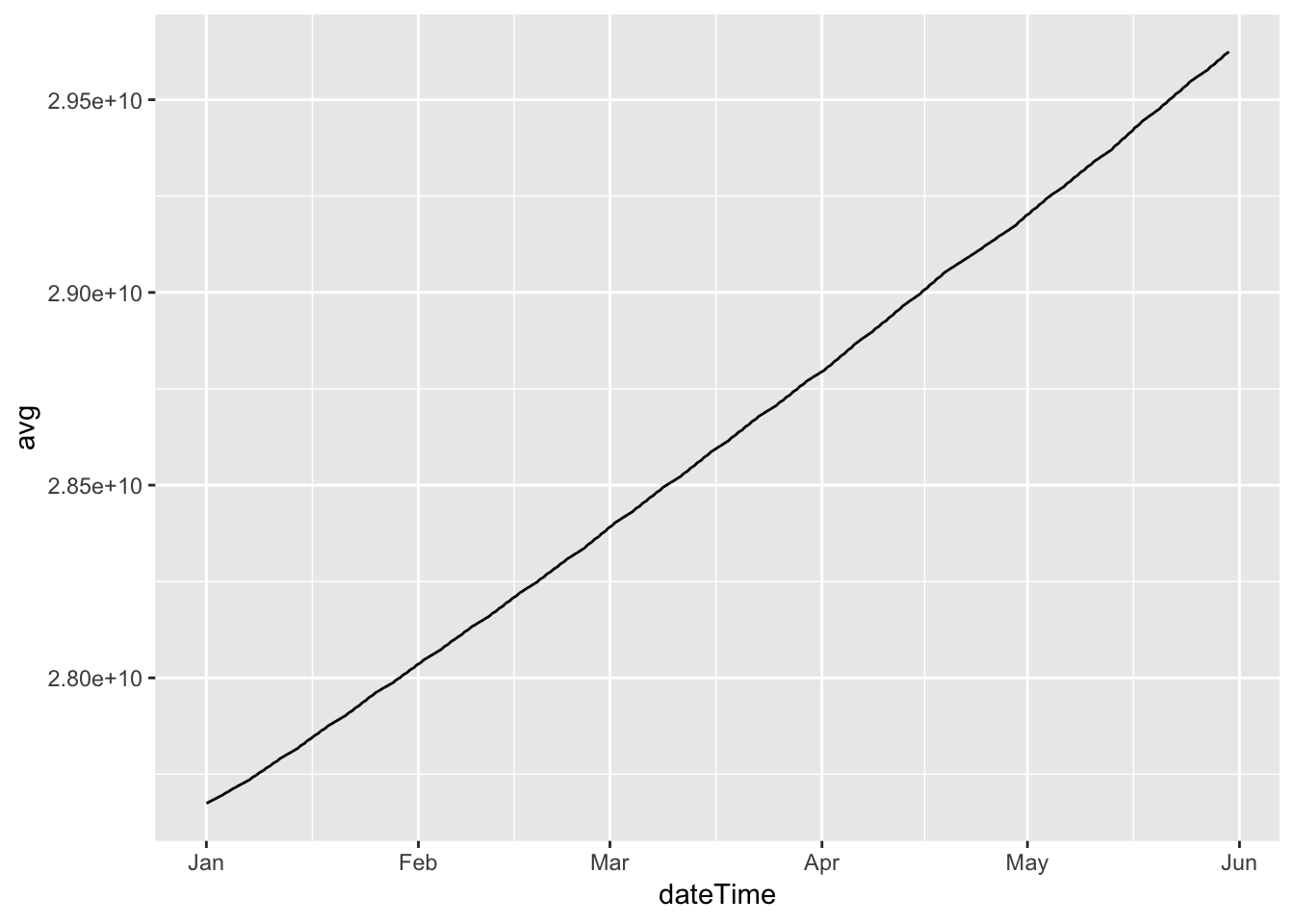
So clearly we have cumulative observations.
4 Test data
Next we calculate the difference making sure the data is sorted by date time and repeat the plot.
setkey(cleanDT, dateTime)
cleanDT[, avgCons := avg - shift(avg)]


p <- ggplot2::ggplot(cleanDT, aes(x = dateTime)) +
  geom_line(aes(y = avgCons))

p
## Warning: Removed 1 rows containing missing values (geom_path).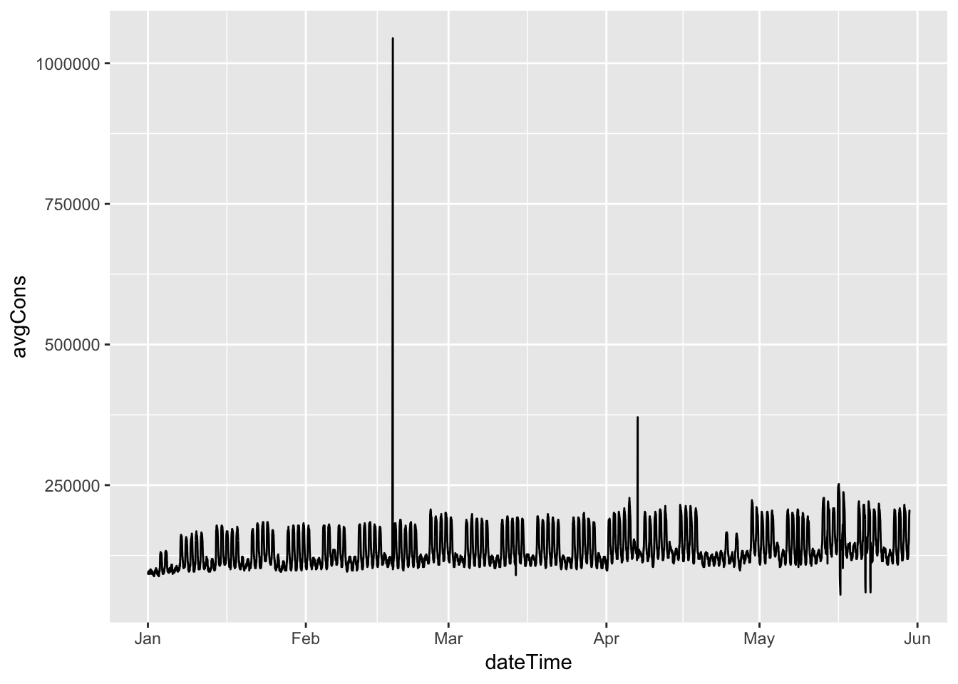
Figure 4.1: Average electricity consumption per 15 minute period
plotly::ggplotly(p) # interactive versionFigure 4.1: Average electricity consumption per 15 minute period
Hmm, clearly some spikes where data has ‘caught up’. We need to check where these data holes might be. The first set of plots summarise the data by date.
plotDT <- cleanDT[, .(nObs = .N,
                      meanCons = mean(avgCons)), keyby = .(date)]
plotDT[, dow := lubridate::wday(date, label = TRUE)]

p <- ggplot2::ggplot(plotDT, aes(x = date, colour = dow)) +
  geom_point(aes(y = nObs))
plotly::ggplotly(p)
p <- ggplot2::ggplot(plotDT, aes(x = date, colour = dow)) +
geom_point(aes(y = meanCons))
plotly::ggplotly(p)Next we look by date and hour of the day.
plotDT <- cleanDT[, .(nObs = .N,
                      meanCons = mean(avgCons)), keyby = .(date, hour)]

myCaption <- "Non-shaded dates indicate missing observations"

ggplot2::ggplot(plotDT, aes(x = date, y = hour, alpha = nObs)) + geom_tile()+
  labs(x = "Date",
       y = "Hour",
       caption = myCaption) +
  guides(alpha = guide_legend(title = "N Obs"))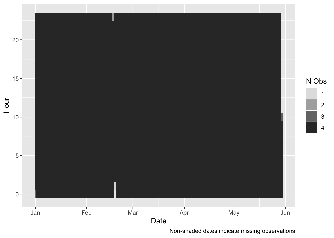
ggplot2::ggplot(plotDT, aes(x = date, y = hour, alpha = meanCons/1000)) + # kWh
  geom_tile() +
  labs(x = "Date",
       y = "Hour",
       caption = myCaption) +
  guides(alpha = guide_legend(title = "Average kWh"))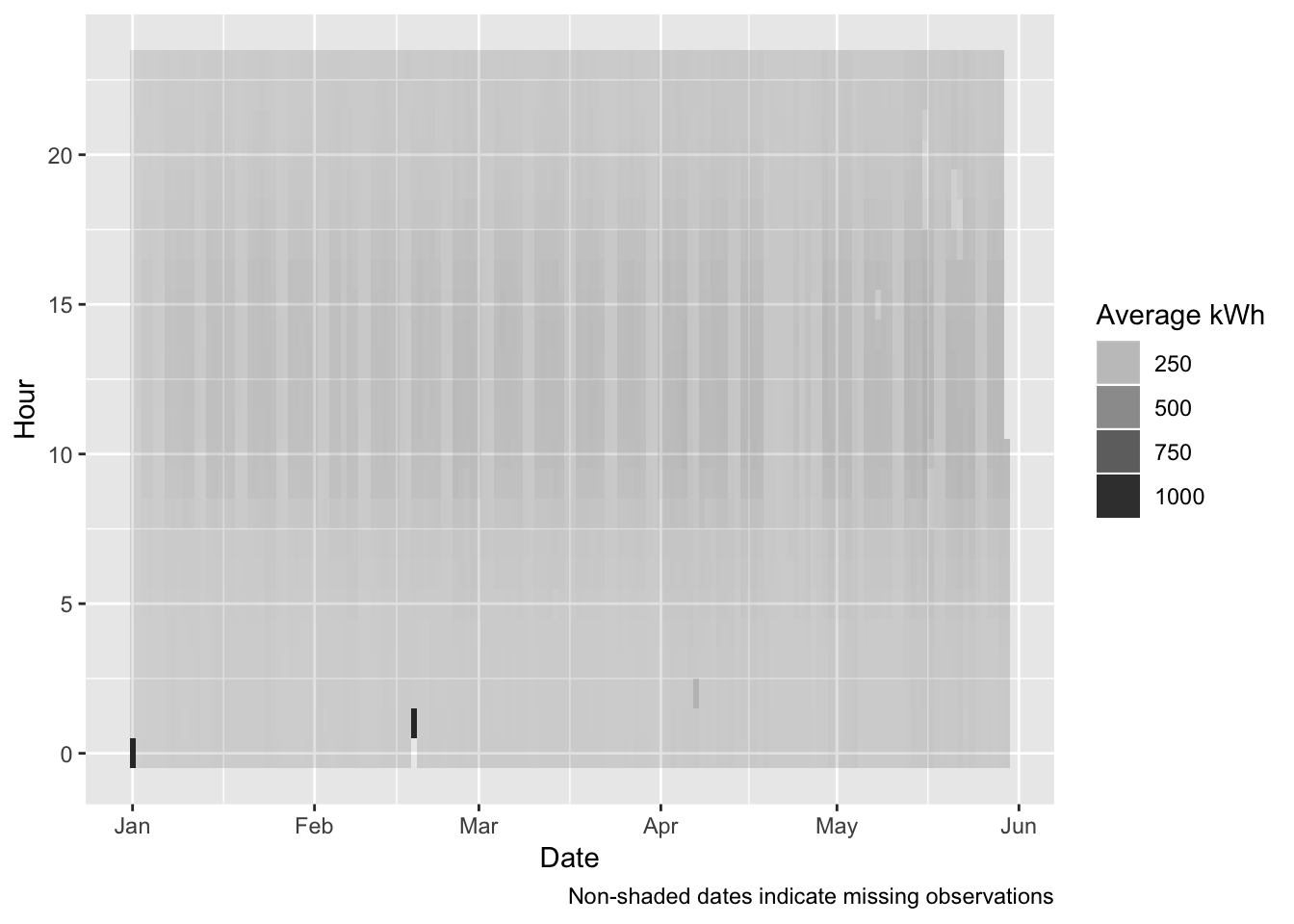
And finally we try to plot all the data to see which observations stand out.
ggplot2::ggplot(cleanDT, aes(x = date, y = hms, alpha = avgCons/1000)) + #kWh
  geom_tile() +
  labs(x = "Date",
       y = "Time of day") +
  guides(alpha = guide_legend(title = "Average kWh"))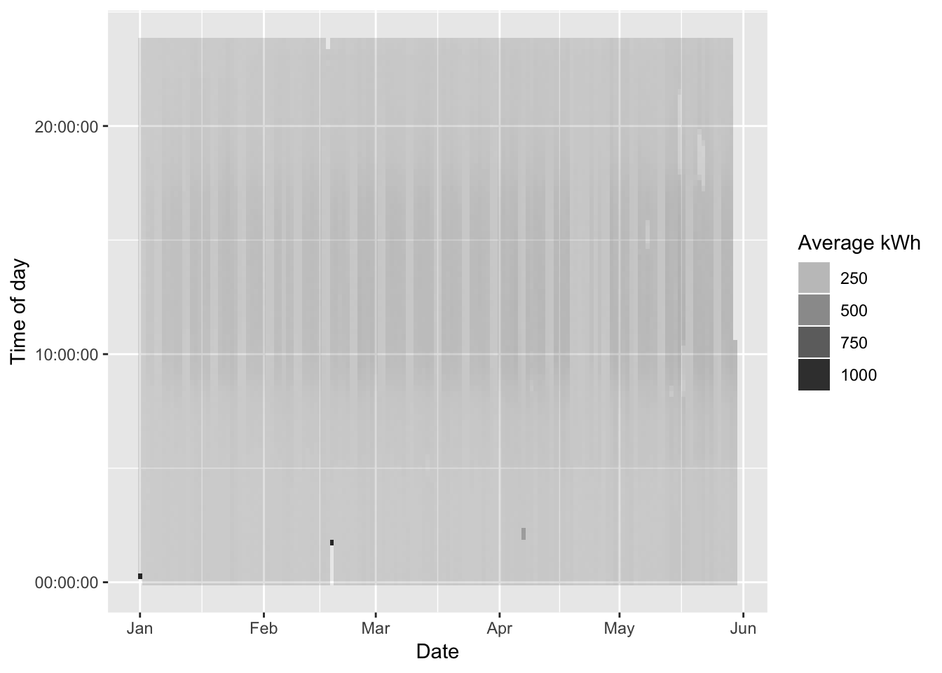
Whats going on? Firstly:
- 7 Apr 2019 - Daylight Saving Time Ended - this will effect observations around 02:00 on Sunday 7th April when there will be a whole hour ‘catch up’. So 8 observations will be allocated to the DST break hour. This means that there will be a mini-spike in apparent consumption;
- 18 Feb 2019 - most likely a data outage causes a ‘catch-up’ spike (see Figure 4.1)
5 Demand profile plots
No data cleaning here. Should remove the 18th Feb data point…
plotDT <- cleanDT[, .(nObs = .N,
                      meanCons = mean(avgCons)), keyby = .(hms, dow, month)]

ggplot2::ggplot(plotDT, aes(x = hms, y = meanCons/1000, colour = dow)) +
  geom_point() +
  facet_grid(month ~ .) +
  labs(y = "kWh per 15 minutes") +
  guides(colour = guide_legend(title = "Day of the week"))
## Warning: Removed 1 rows containing missing values (geom_point).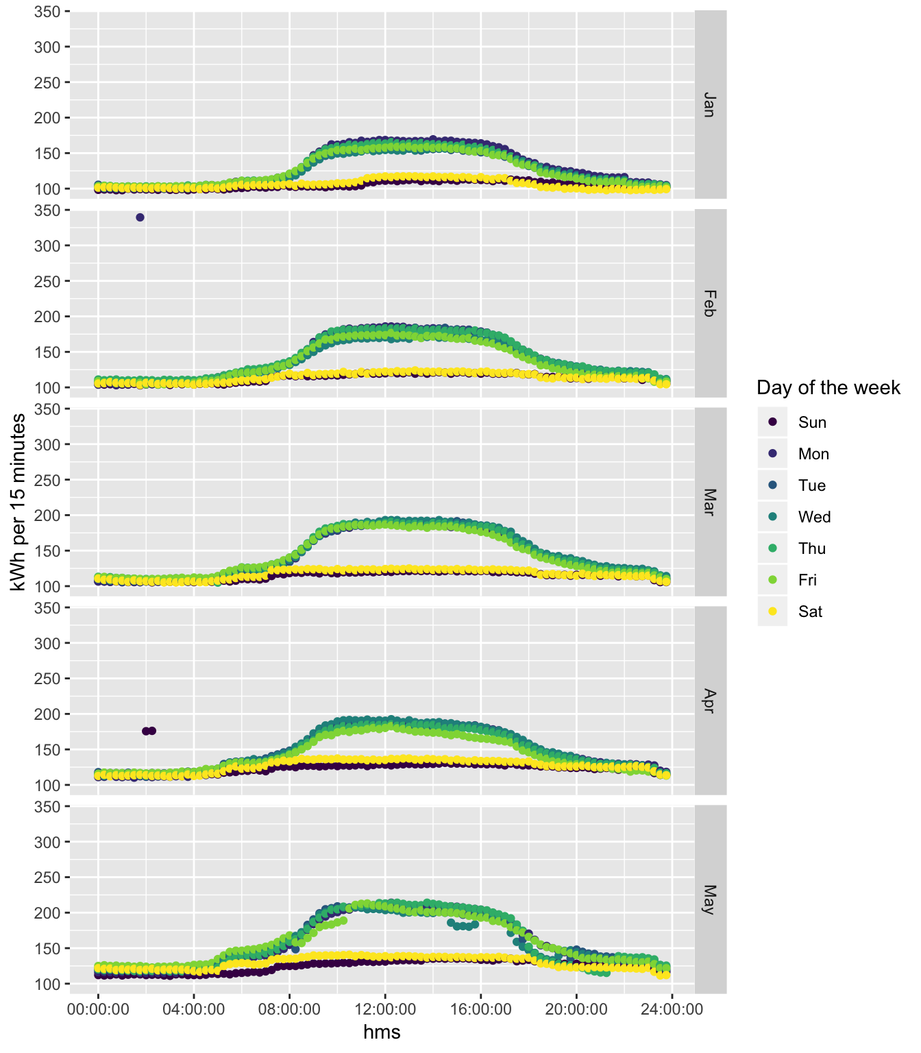
Figure 5.1: Monthly consumption profile plots
And now with the outlier removed…
# just aggregate the data which is less than the max value
plotDT <- cleanDT[avgCons < max(avgCons, na.rm = TRUE), # watch out for the NA
                  .(nObs = .N,
                      meanCons = mean(avgCons)),
                  keyby = .(hms, dow, month)]

ggplot2::ggplot(plotDT, aes(x = hms, y = meanCons/1000, colour = dow)) +
  geom_point() +
  facet_grid(month ~ .) +
  labs(y = "kWh per 15 minutes") +
  guides(colour = guide_legend(title = "Day of the week"))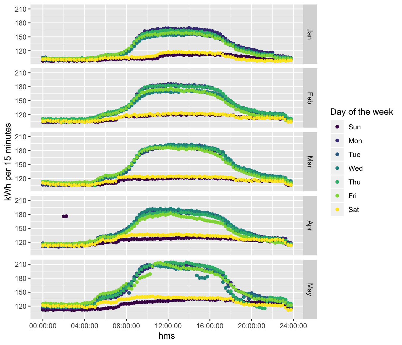
Figure 5.2: Monthly consumption profile plots (Feb 2019 outlier removed)
6 Statistical Annex
Describe the raw data:
skimr::skim(rdt)## Skim summary statistics
## n obs: 14337
## n variables: 24
##
## ── Variable type:character ──────────────────────────────────────────────────────────────────────────────────
## variable missing complete n min max empty n_unique
## Time 0 14337 14337 18 20 0 14337
##
## ── Variable type:integer ────────────────────────────────────────────────────────────────────────────────────
## variable missing complete n mean sd p0 p25 p50 p75 p100
## Number 0 14337 14337 7169 4138.88 1 3585 7169 10753 14337
## hist
## ▇▇▇▇▇▇▇▇
##
## ── Variable type:logical ────────────────────────────────────────────────────────────────────────────────────
## variable missing complete n mean count
## V24 14337 0 14337 NaN 14337
##
## ── Variable type:numeric ────────────────────────────────────────────────────────────────────────────────────
## variable
## Active Energy Total Tariff Sum L1-L3 (30m) [D207 Generator]-avg[Wh]
## Active Energy Total Tariff Sum L1-L3 (30m) [D207 Generator]-max[Wh]
## Active Energy Total Tariff Sum L1-L3 (30m) [D207 Generator]-min[Wh]
## Consumed Active Energy Total Tariff Sum L1-L3 (15m) [D201 and D203 Adams Sayer]-avg[Wh]
## Consumed Active Energy Total Tariff Sum L1-L3 (15m) [D201 and D203 Adams Sayer]-max[Wh]
## Consumed Active Energy Total Tariff Sum L1-L3 (15m) [D201 and D203 Adams Sayer]-min[Wh]
## Consumed Active Energy Total Tariff Sum L1-L3 (15m) [D202 Wellcome]-avg[Wh]
## Consumed Active Energy Total Tariff Sum L1-L3 (15m) [D202 Wellcome]-max[Wh]
## Consumed Active Energy Total Tariff Sum L1-L3 (15m) [D202 Wellcome]-min[Wh]
## Consumed Active Energy Total Tariff Sum L1-L3 (15m) [D204 LFB]-avg[Wh]
## Consumed Active Energy Total Tariff Sum L1-L3 (15m) [D204 LFB]-max[Wh]
## Consumed Active Energy Total Tariff Sum L1-L3 (15m) [D204 LFB]-min[Wh]
## Consumed Active Energy Total Tariff Sum L1-L3 (15m) [D205 Scott]-avg[Wh]
## Consumed Active Energy Total Tariff Sum L1-L3 (15m) [D205 Scott]-max[Wh]
## Consumed Active Energy Total Tariff Sum L1-L3 (15m) [D205 Scott]-min[Wh]
## Consumed Active Energy Total Tariff Sum L1-L3 (15m) [D206 Hercus]-avg[Wh]
## Consumed Active Energy Total Tariff Sum L1-L3 (15m) [D206 Hercus]-max[Wh]
## Consumed Active Energy Total Tariff Sum L1-L3 (15m) [D206 Hercus]-min[Wh]
## Consumed Active Energy Total Tariff Sum L1-L3 (15m) [D20X Whole Medical School]-avg[Wh]
## Consumed Active Energy Total Tariff Sum L1-L3 (15m) [D20X Whole Medical School]-max[Wh]
## Consumed Active Energy Total Tariff Sum L1-L3 (15m) [D20X Whole Medical School]-min[Wh]
## missing complete n mean sd p0 p25
## 13191 1146 14337 1.1e+08 1803061.61 1.1e+08 1.1e+08
## 13191 1146 14337 1.1e+08 1803008.84 1.1e+08 1.1e+08
## 13191 1146 14337 1.1e+08 1803217.58 1.1e+08 1.1e+08
## 0 14337 14337 7.8e+09 1.6e+08 7.6e+09 7.7e+09
## 0 14337 14337 7.8e+09 1.6e+08 7.6e+09 7.7e+09
## 0 14337 14337 7.8e+09 1.6e+08 7.6e+09 7.7e+09
## 0 14337 14337 1.9e+09 4.3e+07 1.9e+09 1.9e+09
## 0 14337 14337 1.9e+09 4.3e+07 1.9e+09 1.9e+09
## 0 14337 14337 1.9e+09 4.3e+07 1.9e+09 1.9e+09
## 0 14337 14337 9.8e+09 1.8e+08 9.5e+09 9.6e+09
## 0 14337 14337 9.8e+09 1.8e+08 9.5e+09 9.6e+09
## 0 14337 14337 9.8e+09 1.8e+08 9.5e+09 9.6e+09
## 0 14337 14337 2.1e+09 4.3e+07 2e+09 2e+09
## 0 14337 14337 2.1e+09 4.3e+07 2e+09 2e+09
## 0 14337 14337 2.1e+09 4.3e+07 2e+09 2e+09
## 1 14336 14337 6.6e+09 1.4e+08 6.4e+09 6.5e+09
## 1 14336 14337 6.6e+09 1.4e+08 6.4e+09 6.5e+09
## 1 14336 14337 6.6e+09 1.4e+08 6.4e+09 6.5e+09
## 0 14337 14337 2.9e+10 5.7e+08 2.8e+10 2.8e+10
## 0 14337 14337 2.9e+10 5.7e+08 2.8e+10 2.8e+10
## 0 14337 14337 2.9e+10 5.7e+08 2.8e+10 2.8e+10
## p50 p75 p100 hist
## 1.1e+08 1.2e+08 1.2e+08 ▇▂▁▁▁▅▁▇
## 1.1e+08 1.2e+08 1.2e+08 ▇▂▁▁▁▅▁▇
## 1.1e+08 1.2e+08 1.2e+08 ▇▂▁▁▁▅▁▇
## 7.8e+09 8e+09 8.1e+09 ▇▇▇▆▆▇▆▆
## 7.8e+09 8e+09 8.1e+09 ▇▇▇▆▆▇▆▆
## 7.8e+09 8e+09 8.1e+09 ▇▇▇▆▆▇▆▆
## 1.9e+09 2e+09 2e+09 ▇▇▇▇▇▇▇▇
## 1.9e+09 2e+09 2e+09 ▇▇▇▇▇▇▇▇
## 1.9e+09 2e+09 2e+09 ▇▇▇▇▇▇▇▇
## 9.8e+09 9.9e+09 1e+10 ▇▇▇▆▆▆▆▆
## 9.8e+09 9.9e+09 1e+10 ▇▇▇▆▆▆▆▆
## 9.8e+09 9.9e+09 1e+10 ▇▇▇▆▆▆▆▆
## 2.1e+09 2.1e+09 2.1e+09 ▇▇▇▇▇▇▆▆
## 2.1e+09 2.1e+09 2.1e+09 ▇▇▇▇▇▇▆▆
## 2.1e+09 2.1e+09 2.1e+09 ▇▇▇▇▇▇▆▆
## 6.6e+09 6.7e+09 6.9e+09 ▇▇▇▇▇▇▇▆
## 6.6e+09 6.7e+09 6.9e+09 ▇▇▇▇▇▇▇▆
## 6.6e+09 6.7e+09 6.9e+09 ▇▇▇▇▇▇▇▆
## 2.9e+10 2.9e+10 3e+10 ▇▇▇▇▇▇▆▆
## 2.9e+10 2.9e+10 3e+10 ▇▇▇▇▇▇▆▆
## 2.9e+10 2.9e+10 3e+10 ▇▇▇▇▇▇▆▆7 Runtime
Analysis completed in 9.62 seconds ( 0.16 minutes) using knitr in RStudio with R version 3.5.2 (2018-12-20) running on x86_64-apple-darwin15.6.0.
8 R environment
R packages used:
- base R - for the basics (R Core Team 2016)
- bookdown - to make the report (Xie 2016)
- data.table - for fast (big) data handling (Dowle et al. 2015)
- hms - clock time (Müller 2018)
- lubridate - date manipulation (Grolemund and Wickham 2011)
- ggplot2 - for slick graphics (Wickham 2009)
- kableExtra - neat tables (Zhu 2018)
- plotly - interactive plots (Sievert et al. 2016)
Session info:
## R version 3.5.2 (2018-12-20)
## Platform: x86_64-apple-darwin15.6.0 (64-bit)
## Running under: macOS High Sierra 10.13.6
##
## Matrix products: default
## BLAS: /Library/Frameworks/R.framework/Versions/3.5/Resources/lib/libRblas.0.dylib
## LAPACK: /Library/Frameworks/R.framework/Versions/3.5/Resources/lib/libRlapack.dylib
##
## locale:
## [1] en_NZ.UTF-8/en_NZ.UTF-8/en_NZ.UTF-8/C/en_NZ.UTF-8/en_NZ.UTF-8
##
## attached base packages:
## [1] stats     graphics  grDevices utils     datasets  methods   base
##
## other attached packages:
## [1] skimr_1.0.5       plotly_4.9.0      lubridate_1.7.4   kableExtra_1.1.0
## [5] hms_0.4.2         ggplot2_3.1.1     data.table_1.12.2
##
## loaded via a namespace (and not attached):
##  [1] tidyselect_0.2.5  xfun_0.7          reshape2_1.4.3
##  [4] purrr_0.3.2       colorspace_1.4-1  htmltools_0.3.6
##  [7] viridisLite_0.3.0 yaml_2.2.0        rlang_0.3.4
## [10] pillar_1.4.1      later_0.8.0       glue_1.3.1
## [13] withr_2.1.2       plyr_1.8.4        stringr_1.4.0
## [16] munsell_0.5.0     gtable_0.3.0      rvest_0.3.3
## [19] htmlwidgets_1.3   evaluate_0.13     labeling_0.3
## [22] knitr_1.23        httpuv_1.5.1      crosstalk_1.0.0
## [25] highr_0.8         Rcpp_1.0.1        xtable_1.8-4
## [28] readr_1.3.1       scales_1.0.0      promises_1.0.1
## [31] webshot_0.5.1     jsonlite_1.6      mime_0.6
## [34] digest_0.6.19     stringi_1.4.3     bookdown_0.10
## [37] dplyr_0.8.1       shiny_1.3.2       grid_3.5.2
## [40] cli_1.1.0         tools_3.5.2       magrittr_1.5
## [43] lazyeval_0.2.2    tibble_2.1.2      crayon_1.3.4
## [46] tidyr_0.8.3       pkgconfig_2.0.2   xml2_1.2.0
## [49] assertthat_0.2.1  rmarkdown_1.13    httr_1.4.0
## [52] rstudioapi_0.10   R6_2.4.0          compiler_3.5.2
References
Dowle, M, A Srinivasan, T Short, S Lianoglou with contributions from R Saporta, and E Antonyan. 2015. Data.table: Extension of Data.frame. https://CRAN.R-project.org/package=data.table.
Grolemund, Garrett, and Hadley Wickham. 2011. “Dates and Times Made Easy with lubridate.” Journal of Statistical Software 40 (3): 1–25. http://www.jstatsoft.org/v40/i03/.
Müller, Kirill. 2018. Hms: Pretty Time of Day. https://CRAN.R-project.org/package=hms.
R Core Team. 2016. R: A Language and Environment for Statistical Computing. Vienna, Austria: R Foundation for Statistical Computing. https://www.R-project.org/.
Sievert, Carson, Chris Parmer, Toby Hocking, Scott Chamberlain, Karthik Ram, Marianne Corvellec, and Pedro Despouy. 2016. Plotly: Create Interactive Web Graphics via ’Plotly.js’. https://CRAN.R-project.org/package=plotly.
Wickham, Hadley. 2009. Ggplot2: Elegant Graphics for Data Analysis. Springer-Verlag New York. http://ggplot2.org.
Xie, Yihui. 2016. Bookdown: Authoring Books and Technical Documents with R Markdown. Boca Raton, Florida: Chapman; Hall/CRC. https://github.com/rstudio/bookdown.
Zhu, Hao. 2018. KableExtra: Construct Complex Table with ’Kable’ and Pipe Syntax. https://CRAN.R-project.org/package=kableExtra.